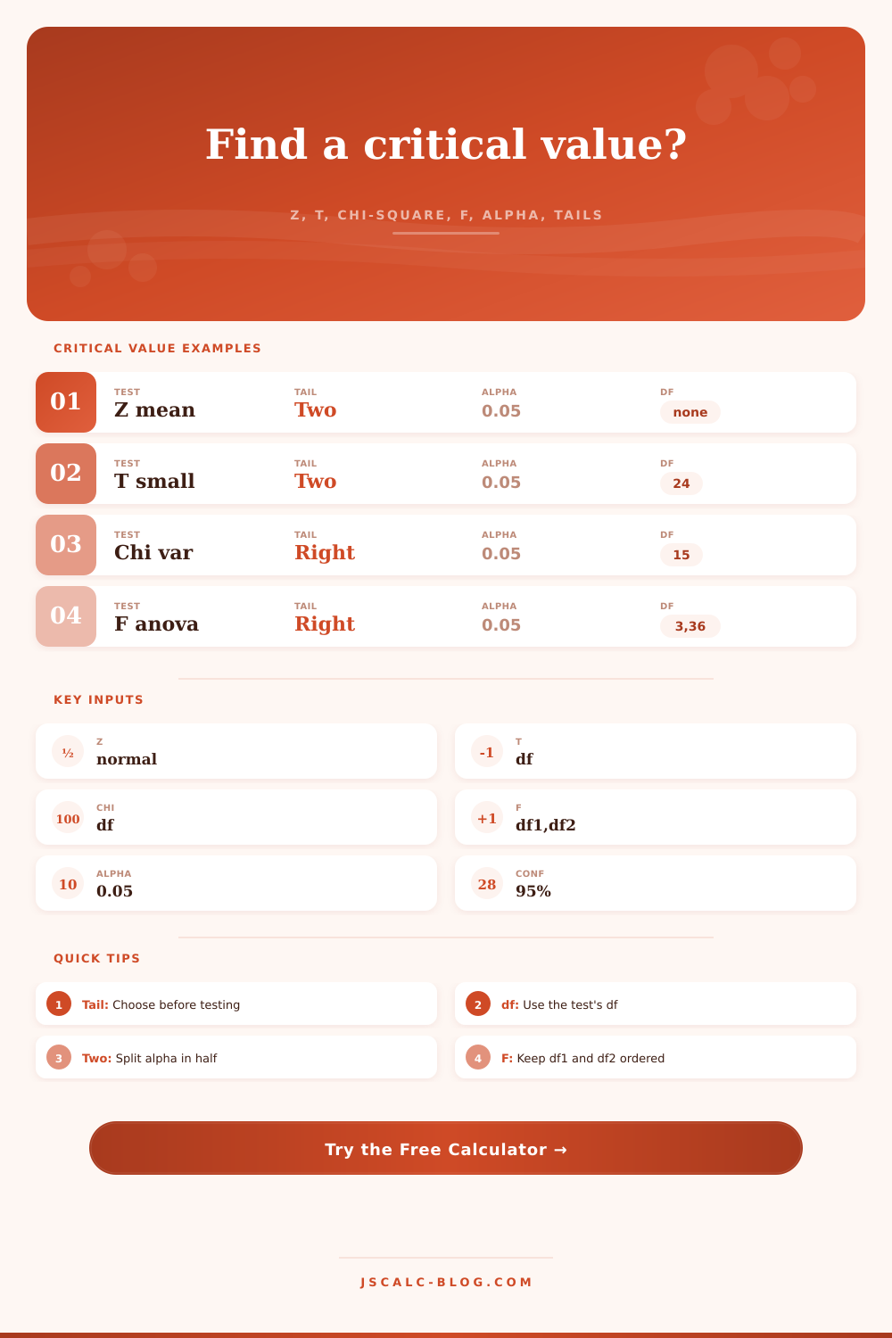
Critical Value Calculator
Find critical cutoffs for normal z, Student t, chi-square, and F distributions using alpha, tail direction, degrees of freedom, and confidence level.
Load a common hypothesis-test or interval setup, then adjust alpha, tails, degrees of freedom, or confidence level.
Enter distribution settings to calculate critical values.
| Distribution | Setup | Alpha or confidence | Lower critical | Upper critical |
|---|---|---|---|---|
| Z | Two-tailed | 0.05 | -1.960 | 1.960 |
| Confidence level | Total alpha | Two-tailed z | One-sided alpha | One-sided z |
|---|---|---|---|---|
| 80% | 0.20 | +/- 1.282 | 0.20 | 0.842 |
| 90% | 0.10 | +/- 1.645 | 0.10 | 1.282 |
| 95% | 0.05 | +/- 1.960 | 0.05 | 1.645 |
| 98% | 0.02 | +/- 2.326 | 0.02 | 2.054 |
| 99% | 0.01 | +/- 2.576 | 0.01 | 2.326 |
| 99.9% | 0.001 | +/- 3.291 | 0.001 | 3.090 |
| Test or interval | Distribution | Typical tail | Degrees of freedom | Critical value cue |
|---|---|---|---|---|
| Population mean, known sigma | Z | Two or one | None | Use standard normal cutoffs. |
| One-sample or paired mean | t | Two or one | n - 1 | Small df makes larger cutoffs. |
| Welch two-sample mean | t | Two or one | Welch df | Fractional df is allowed. |
| Variance upper-tail test | Chi-square | Right | n - 1 | Reject for large chi-square. |
| Variance confidence interval | Chi-square | Two bounds | n - 1 | Use both lower and upper chi-square values. |
| ANOVA factor test | F | Right | df1, df2 | Reject for large F ratios. |
| Variance ratio test | F | Two bounds | n1 - 1, n2 - 1 | Order the numerator variance first. |
| Regression overall F | F | Right | p, n - p - 1 | Use model df over error df. |
If you’ve taken most statistics classes, you’re familiar with determining p-values; not so much with the limits upon which their significance depend. Enter: the critical value. That’s the number where random chance ends and something meaningful emerge. Without it, you’d have no idea if what you found was an actual thing or just good fortune.
Once you input your distribution type and tail direction, the calculator do all the math for you. No need to remember (or flip through heavy textbooks’ appendices) for numbers based off different sample size. The tool accounts for degrees of freedom.
Understanding Critical Values
The most basic place to begin is normal distribution. In this case, you’re dealing with a z-score, which means you have a known population standard deviation and are interested in testing a mean. At the five percent significance level for a standard two-tailed test, the critical values is ±1.96. If your test statistic is beyond those bounds, then you reject the null hypothesis.
That’s a hard-and-fast rule, but it works because the normal curve is so predictable and symmetrical. You don’t have to worry about sample size skewing the shape of the distribution as you would with some of the other tests.
When we advance to the t-distribution (when you’re dealing with a small sample and the population standard deviation are unknown), it becomes more complicated. One major factor in determining the critical value is degrees of freedom (typically equal to sample size, 1). As sample size decreases, the degrees of freedom decrease, making the t-distribution have heavier tails to accomodate additional uncertainty. This causes the critical values to be farther away from zero.
What was a significant test statistic for a large sample may fall below the cut-off point for a small sample. That’s the price you should of pay for insufficient data. These numbers shift constantly depending on the degrees of freedom that you select, illustrating precisely what happens when the threshold becomes tighter or looser.
The chi-square distribution is totally new to variance testing; it’s not symmetric like your t and z tests. Instead, the chi-square distribution lean to the right (with zero as the lower bound). Why does this matter? You can’t have negative variance. So when you’re testing if a variance increase, you examine the right tail. The critical value will be positive.
In contrast, if you’re building a confidence interval around variance, you require two critical values: one for each end of the interval. The upper bound will use a low percentile of the distribution, whereas the lower bound will use a high one. At first, this seems counterintuitive, but the math take into account the curve’s skewness.
For example, with an ANOVA (comparing multiple groups), or to test the variance between two thing, we use the F-distribution. You compare your result to a critical value from this distribution using two degrees of freedom, one for the numerator and another for the denominator. Which comes first? Switching their orders yields completely different results.
Because you’re trying to find a big number (a ratio much higher than 1) the majority of ANOVAs is considered right-tailed tests. If your ratios are all about the same as each other, they’ll cluster around a ratio of 1. The bigger the F-value, the more likely it is that the group means is different. The calculator will crunch those numbers and return the final answer. This saves us the headache of looking up values in two separate columns of degrees of freedom tables and figuring it out ourselves.
The most frequent error is probably choosing the right tail. You have to choose it based on your alternative hypothesis before looking at the data. If you use a two tailed test, half the alpha gets split across both tails of the distribution. The result is each tail has lower area, so it’s more difficult to reject the null hypothesis.
If instead you do a one tailed test, you place all the alpha on just one side. This decreases the critical value and makes the test more sensitive in that direction, but you lose the ability to detect an effect the other way. That’s the tradeoff: more protection from false positives in the wrong direction than it becomes more sensitive.
These numbers define the line in the sand. They’re not just a pass-fail test; they represent the understanding of your particular context and what constitutes evidence there. The line in the sand… Whether it’s a manufacturing tolerance check, or an audit of your finances (that’s the number to know).
Now you have your rules set. Now the data talks. All you have to do is figure out where to draw the line.