Sample Size for Comparing Two Means Calculator
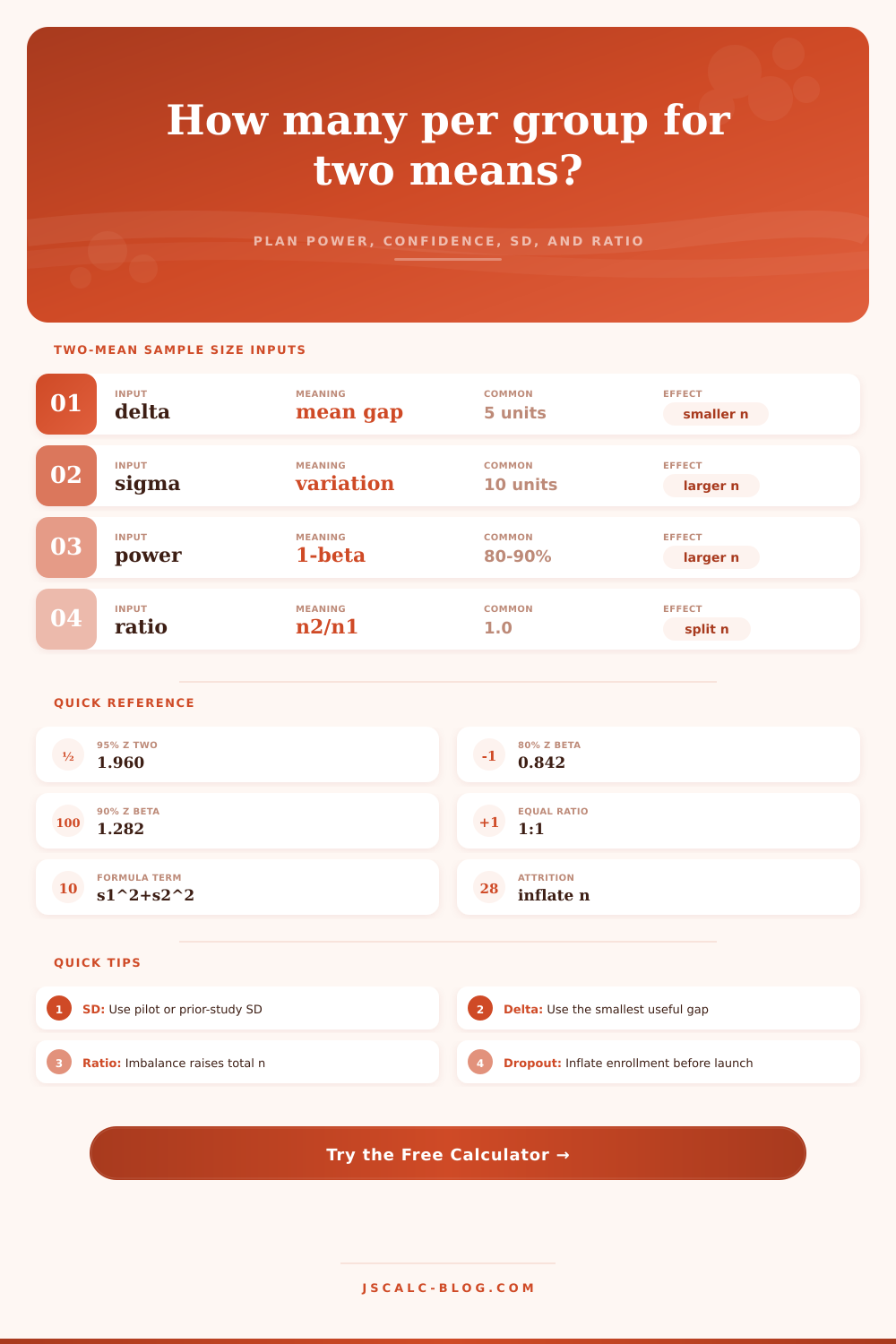
Plan the sample size needed to compare two independent means with known or planning standard deviations. Enter the minimum detectable difference, confidence level, target power, allocation ratio, and dropout allowance to get analyzed and enrollment sample sizes.
🎯Two-Mean Study Presets
📝Sample Size Inputs
Two-sided designs use z alpha/2; one-sided designs use z alpha.
Confidence converts to alpha = 1 - confidence.
Power = 1 - beta, the chance of detecting the chosen difference.
Use the smallest difference worth detecting, in outcome units.
Control or reference group standard deviation.
Treatment or comparison group standard deviation.
Set 1 for equal groups; 2 gives twice as many in group 2.
Enrollment n is inflated by 1 / (1 - dropout).
🔢Current Design Snapshot
⚙Formula Breakdown
📊Confidence and Power Z Reference
| Setting | Alpha or Beta | Two-Sided z | One-Sided z | Planning Effect | Common Use |
|---|---|---|---|---|---|
| 90% confidence | alpha 0.10 | 1.645 | 1.282 | Lowest n | Early screen |
| 95% confidence | alpha 0.05 | 1.960 | 1.645 | Standard n | Common study |
| 99% confidence | alpha 0.01 | 2.576 | 2.326 | Higher n | Strict evidence |
| 80% power | beta 0.20 | 0.842 | 0.842 | Common target | Feasible plan |
| 90% power | beta 0.10 | 1.282 | 1.282 | Higher n | Lower miss risk |
| 95% power | beta 0.05 | 1.645 | 1.645 | Largest n | High assurance |
⚖Allocation Ratio Reference
| k = n2/n1 | Group 2 Share | Variance Term | Efficiency | When It Fits | Caution |
|---|---|---|---|---|---|
| 0.25 | 20% | s1² + 4s2² | Low | Rare treatment data | Large group 1 needed |
| 0.50 | 33% | s1² + 2s2² | Moderate | Limited group 2 | Total n rises |
| 1.00 | 50% | s1² + s2² | Highest | Equal cost arms | Best default |
| 1.50 | 60% | s1² + 0.67s2² | High | More treatment exposure | Small efficiency loss |
| 2.00 | 67% | s1² + 0.5s2² | Moderate | Safety or rollout reasons | Control gets thinner |
| 4.00 | 80% | s1² + 0.25s2² | Low | Strong preference for group 2 | Often costly overall |
🧪Study Scenario Comparison Grid
| Scenario | Delta | Sigma1 | Sigma2 | Ratio k | Confidence | Power | Dropout | Typical Read |
|---|---|---|---|---|---|---|---|---|
| Blood pressure trial | 5 mmHg | 12 | 12 | 1.00 | 95% | 80% | 10% | Clinical difference |
| Website latency test | 35 ms | 90 | 85 | 1.00 | 95% | 90% | 2% | Performance shift |
| Class score comparison | 4 points | 9 | 10 | 1.00 | 95% | 80% | 5% | Education outcome |
| Package fill weight | 1.5 g | 3.2 | 3.0 | 1.00 | 99% | 90% | 1% | Quality control |
| Unequal clinic arms | 3 units | 8 | 9 | 1.50 | 95% | 85% | 15% | More treatment slots |
| Battery life comparison | 1.2 hours | 2.5 | 2.8 | 1.00 | 95% | 90% | 0% | Product testing |
| Training time reduction | 6 minutes | 18 | 16 | 2.00 | 95% | 80% | 8% | Operational rollout |
| Survey scale shift | 0.35 points | 1.1 | 1.0 | 1.00 | 90% | 80% | 12% | Attitude change |
📐Effect Size Planning Table
| Standardized Gap | Delta if SD 10 | Planning Label | n Pressure | Design Note |
|---|---|---|---|---|
| 0.10 | 1 point | Very small | Very high | Needs precise measurement |
| 0.20 | 2 points | Small | High | Often large studies |
| 0.50 | 5 points | Moderate | Moderate | Common planning anchor |
| 0.80 | 8 points | Large | Lower | Usually easier to detect |
| 1.00 | 10 points | Very large | Low | Confirm realism carefully |
💡Sample Size Planning Tips
The hypothesis is that your new teaching method boosts test scores. Time to prove it! You’re ready with the data, enthusiasm, and determination. You probably don’t have one thing: patience for collecting enough evidence to nail down the point.
If you fails to plan your sample size, your study’s outcome will be swamped by noise, and your potential career-changing discovery will go unnoticed. To avoid this, most researchers charge ahead without first running the math. They eventually realize they didn’t run a large enough study to pick up on their actualy effect.
How to Choose the Right Sample Size
The calculator above spares you from guessing about confidence intervals and standard deviations. All you need are your particular assumptions, and the calculator do the grunt work behind this calculation for you.
Every two-group comparison boils down to one thing: How much variation exist in your data vs. How big an effect do you care about? Do you have blood pressure numbers? Those will bounce all over the place for different patient. Are you weighing a manufactured widget? Maybe the variation is minuscule. That’s what the tool reflects based off its standard deviation inputs.
In almost every case, your biggest mistake will be to underestimate the variation. You may start with overly rosy numbers from a pilot study with favorable conditions, making it seem like you will needed a reasonable sample size. Then the real world intrudes. All that noise drowns out the signal. Be conservative here; it pays.
And then there’s power. Power is a fancy word meaning “the probability that you’ll detect an effect if it actualy does exist.” Why is it set at eighty percent? That is the sweet spot. We know this because it is where the industry has landed after weighing the cost of gathering data against the risk of missing something important if you push too low. Ninety percent or even eighty-five percent might sound good, but it can translate into sample sizes that is impossible to recruit. The table on the page makes this clear: Small changes to those targets mean huge changes in required headcounts.
What type of error can you tolerate? The other tool folks tend to overlook is the allocation ratio. This is the assumption that most efficient groups are always of equal sizes. That’s true, by definition, if you’re trying to be efficient. But in the real world, things aren’t always equal. Perhaps your treatment arms don’t has equal numbers (for example, because there’s only a small number of participants available for one arm). Or perhaps you know that one of these treatments is scarce or expensive. In that case you can change the ratio in the tool to account for this difference.
The tradeoff? Total sample size. Typically, unbalanced group require greater total sample size to get the same statistical power. So it’s an element of both math and logistics.
And don’t neglect the dropout rate. That’s the less sexy aspect of study design that sends more studies down the toilet than faulty hypotheses do. Machines fail, people drop out, data becomes corrupt. If you think 10% will drop out, and you’re planning on enrolling 50 per arm, you should of begin with 56. It sucks to have to repeat the study because you didn’t pad your enrollment enough. The calculator does that padding for you, it inflates the sample sizes automatically. It is a big help.
In the end, this is all about being honest with yourself. Sample size planning makes you say exactly what difference you care about, and how sure you need to be that it’s there. Maybe you’ll find out that you need a sample of three thousand people. Maybe your effect size isn’t big enough to even care about. Or maybe your variance is too large to be measured reliablly. The math doesn’t judge. It merely shows the price tag on your ambitions.
Plan carefully ahead so as not to ruin your credibility down the road. You don’t want your results drowning in the static of a poorly powered study, you want them to speak for themselves. Get your numbers right before you start.