Throughput Calculator
Work out achievable network throughput two ways: from data transferred over elapsed time, or from a TCP window over the round trip time when the window is the limit. Then see goodput after protocol overhead, efficiency against the link capacity, and how long a target file will take to move.
📡Choose a Method
🎯Real Throughput Presets
📝Throughput Inputs
Total payload moved during the measured transfer.
Bytes and bits are both supported here.
How long the transfer took, in the unit below.
Applies to the elapsed time field.
Receive window advertised, in kilobytes (1 KB = 1024 B).
Ping time for one round trip in milliseconds.
Headers plus retransmits removed to get goodput.
Rated line rate, used for the efficiency card.
File size for the time-to-transfer estimate.
Unit for the target transfer size above.
🔢Formula Snapshot
📊Window and RTT to Max Throughput
| TCP Window | RTT 10 ms | RTT 20 ms | RTT 50 ms | RTT 100 ms | RTT 200 ms |
|---|---|---|---|---|---|
| 16 KB | 13.1 Mbps | 6.6 Mbps | 2.6 Mbps | 1.3 Mbps | 0.7 Mbps |
| 32 KB | 26.2 Mbps | 13.1 Mbps | 5.2 Mbps | 2.6 Mbps | 1.3 Mbps |
| 64 KB | 52.4 Mbps | 26.2 Mbps | 10.5 Mbps | 5.2 Mbps | 2.6 Mbps |
| 128 KB | 104.9 Mbps | 52.4 Mbps | 21.0 Mbps | 10.5 Mbps | 5.2 Mbps |
| 256 KB | 209.7 Mbps | 104.9 Mbps | 41.9 Mbps | 21.0 Mbps | 10.5 Mbps |
| 512 KB | 419.4 Mbps | 209.7 Mbps | 83.9 Mbps | 41.9 Mbps | 21.0 Mbps |
| 1 MB | 838.9 Mbps | 419.4 Mbps | 167.8 Mbps | 83.9 Mbps | 41.9 Mbps |
| 2 MB | 1677.7 Mbps | 838.9 Mbps | 335.5 Mbps | 167.8 Mbps | 83.9 Mbps |
📋Typical Protocol Overhead
| Scenario | Header Overhead | With Resends | Goodput of 100 Mbps |
|---|---|---|---|
| TCP over Ethernet 1500 MTU | ~3.7% | ~5-7% | ~94 Mbps |
| TCP with jumbo 9000 MTU | ~0.6% | ~2-3% | ~97 Mbps |
| IPsec VPN tunnel | ~8-10% | ~12-15% | ~85 Mbps |
| Wi-Fi with MAC layer | ~15-25% | ~30-45% | ~60 Mbps |
| Small packet VoIP mix | ~30-50% | ~35-55% | ~50 Mbps |
| Lossy WAN 1% loss | ~4% | ~20-40% | ~65 Mbps |
📡Real World Efficiency by Link Type
| Link Type | Rated Rate | Typical Throughput | Efficiency |
|---|---|---|---|
| Gigabit Ethernet | 1000 Mbps | 930-945 Mbps | 93-95% |
| Fast Ethernet | 100 Mbps | 92-95 Mbps | 92-95% |
| Wi-Fi 6 (real) | 1200 Mbps | 500-700 Mbps | 42-58% |
| Wi-Fi 5 (real) | 866 Mbps | 300-450 Mbps | 35-52% |
| Cable DOCSIS 3.1 | 500 Mbps | 440-490 Mbps | 88-98% |
| ADSL2+ down | 24 Mbps | 18-22 Mbps | 75-92% |
| 4G LTE | 100 Mbps | 20-50 Mbps | 20-50% |
| GEO Satellite | 50 Mbps | 15-35 Mbps | 30-70% |
🗃Method Comparison Grid
| Method | Formula | Limiting Factor | Typical Result | Best Use |
|---|---|---|---|---|
| Data over time | bits / seconds | Whatever the bottleneck is | Actual measured Mbps | Post transfer audit |
| TCP window / RTT | win x 8 / RTT | Receive window and latency | Window capped ceiling | Long fat WAN links |
| Goodput | T x (1 - overhead) | Headers and retransmits | Payload only rate | App layer planning |
| Efficiency | T / link x 100 | Protocol and medium | 40% to 95% | Comparing links |
| Time to transfer | size x 8 / T | Sustained throughput | Seconds to hours | Backup windows |
📏Data and Rate Unit Reference
| Unit | Equals | In Bits | Note |
|---|---|---|---|
| 1 byte | 8 bits | 8 b | Files are bytes |
| 1 KB | 1024 bytes | 8192 b | Binary kilobyte |
| 1 MB | 1024 KB | 8.39 million b | Binary megabyte |
| 1 GB | 1024 MB | 8.59 billion b | Binary gigabyte |
| 1 Mbps | 0.125 MB/s | 1 million b/s | Link rates in bits |
| 1 Gbps | 125 MB/s | 1 billion b/s | Decimal for lines |
⚙Formula Breakdown
💡Throughput Reality Tips
Throughput is how much data really goes across your network. It is not what’s printed on the box. It’s rare for a 1000 Mbps link to deliver that many megabits/second when you’re transferring files. Latency and window size can slows down even a fast fiber circuit. The calculator figures out what you’ll achieve two ways. It then converts that to a realistic transfer time, along with how efficient your connection was (goodput), so you can calculate backup times with numbers you can defend.
There are two way: The most direct way is data over time. How many bits did you move in how much time? Total bits over the seconds equals your throughput. That’s what measured mode tell you, after the fact. It’s the honest figure that already factors in the cause of your slower-than-maximum transfer, whether the disk was too slow or the network were congested.
Understanding Real Network Speeds
The other figures out a theoretical limit ahead of time. In order for a TCP connection to work at all, there can never be more than one window’s worth of data outstanding at any moment during a round trip. So, the maximum rate you’ll see is your window in bits divided by your round trip time. For long distance links this makes an enormous difference. In these cases the window size and the large round trip time combine to cap the rate well below line speed, but silently.
Network people say things are “bits” per second. File transfer stats on your OS show them as being “bytes” per second. But there’s a difference: eight times different than. One megabyte per second equals eight megabits per second. Eight megabytes is equal to one gigabyte. And so on. This means that a 100 Mbps internet connection is going to bring you a top speed of roughly 12.5 MB/s. That’s why it takes more like 86 seconds to download a one gigabyte file, not ten seconds (assuming a perfect line). The calculator removes this common point of confusion by handling either unit as input.
So what’s on the other end of this? That’s raw throughput: every bit that goes across the wire. But most of it isn’t your own payload; much of it is just protocol headers or even retransmissions. The useful fraction that gets to the application is called goodput. Here we subtract the overhead. Standard framing wastes a few percent in Ethernet. An IPsec VPN tunnel adds another eight to fifteen percent. Wi-Fi can lose twenty to forty percent thanks to all that media access control and collision handling. If you’re on a lossy path then retransmissions will dominate. So despite the line looking okay from above, goodput can colapse.
Throughput divided by capacity is called efficiency. It’s measured in percentages. 93 to 95 percent is common for well tuned wired gigabit connections. That means 940 Mbps on a 1000 Mbps port are healthy. By comparison, real world Wi-Fi can land anywhere from forty to sixty percent of its advertised rate. Why? Because that rate is a theoretical physical layer maximum under ideal conditions. Efficiency converts a raw rate into a judgment: Is this link performing as it should of be?
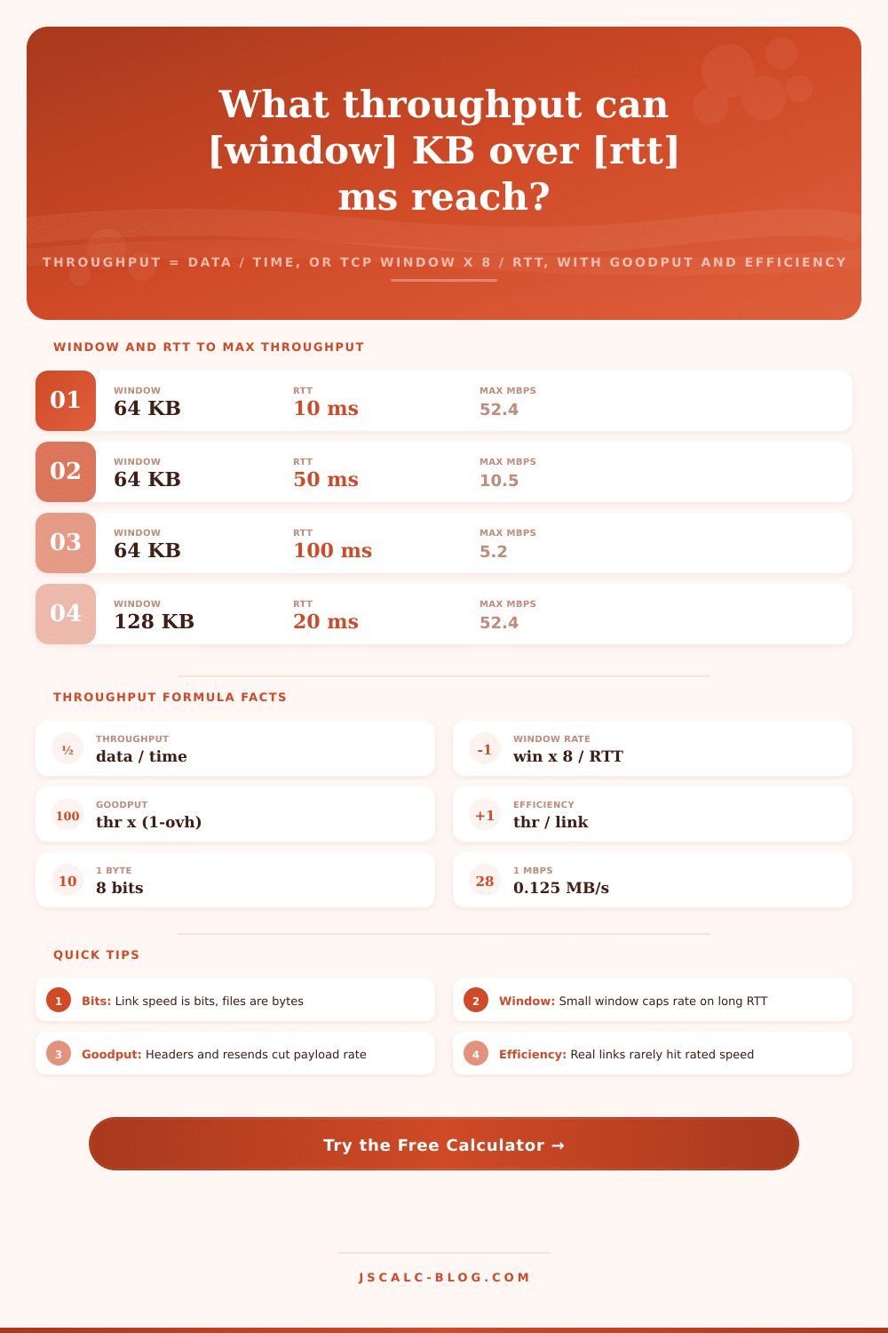
But the relationship between window and round trip times exposes the latency trap rapidly. Go down one row of the window sizes and then across the delay columns. Every doubling of round trip cuts the achievable throughput in half. At 10ms it’s ~52 Mbps with a 64 KB window. But at 100 ms it’s just 5.2 Mbps. So yeah, a transfer from two continents can be slow… even on premium circuits.
And how do we fix this? A bigger window. Moddern scaling allows exactly this.
If you know the sustained throughput, the time required to move a target file is simply the file’s size in bits divided by that rate. And this is what really matters when thinking about a data center migration or a nightly backup window. You can quickly pick a scenario from the presets to run a test case without having to type in any numbers yourself. Everything from a high latency satellite case down to a gigabit Ethernet copy. And all triggered into full calculation immediatly. This gives you something to start tweaking with your own estimated overheads and data.
Tweak modes: Compare running the measurement against the maximum capacity allowed by the window on the same path. Then you’ll know at a glance what’s really constraining… Latency or the link? It is a small thing, but it matters if you’re planning a big transfer.
So if you know the distinction between rated speed vs. Real throughput, you’ll stop laying blame on the network when in fact it’s a matter of your configuration. You can adjust your windows, select more appropriate protocols, or maybe just pick off-peak times to do your transfers. Speed isn’t everything. Understanding why something’s moving as it is is the point. That’s what throughputs are for: The truth about the marketing numbers. Knowing how to measure it right will save you frustration, and time.