T-Score Calculator
Convert a raw score into a T-score, z-score, normal percentile, classification band, comparison distribution result, and target raw score.
Use the same reference group for raw score, mean, and standard deviation. The comparison fields translate the same standing onto another distribution.
| T-score band | z range | Percentile range | Common label | Quick read |
|---|---|---|---|---|
| 70 and above | +2.00 or more | 97.7%+ | Very high | Far above the mean |
| 60 to 69.9 | +1.00 to +1.99 | 84.1% to 97.6% | High | Above typical range |
| 55 to 59.9 | +0.50 to +0.99 | 69.1% to 83.9% | High average | Somewhat above mean |
| 45 to 54.9 | -0.50 to +0.49 | 30.9% to 69.1% | Average | Close to mean |
| 40 to 44.9 | -1.00 to -0.51 | 15.9% to 30.5% | Low average | Somewhat below mean |
| 30 to 39.9 | -2.00 to -1.01 | 2.3% to 15.7% | Low | Below typical range |
| Below 30 | Below -2.00 | Below 2.3% | Very low | Far below the mean |
| z-score | T-score | Percentile | Raw formula | Interpretation |
|---|---|---|---|---|
| -2.00 | 30 | 2.3% | mean - 2SD | Very low tail |
| -1.50 | 35 | 6.7% | mean - 1.5SD | Low |
| -1.00 | 40 | 15.9% | mean - 1SD | Below average |
| -0.50 | 45 | 30.9% | mean - 0.5SD | Low average |
| 0.00 | 50 | 50.0% | mean | Average |
| +0.50 | 55 | 69.1% | mean + 0.5SD | High average |
| +1.00 | 60 | 84.1% | mean + 1SD | High |
| +1.50 | 65 | 93.3% | mean + 1.5SD | Very high |
| +2.00 | 70 | 97.7% | mean + 2SD | Upper tail |
| Use case | Raw score | Mean | SD | T-score | Percentile |
|---|---|---|---|---|---|
| Class exam | 84 | 70 | 10 | 64.0 | 91.9% |
| Clinical scale | 72 | 50 | 10 | 72.0 | 98.6% |
| Reading norm | 108 | 100 | 15 | 55.3 | 70.3% |
| Athletic test | 38 | 45 | 7 | 40.0 | 15.9% |
| Hiring screen | 62 | 55 | 6 | 61.7 | 87.8% |
| Quality audit | 9.8 | 10.5 | 0.4 | 32.5 | 4.0% |
| Comparison task | Distribution A | Distribution B | Shared value | Method |
|---|---|---|---|---|
| Translate same standing | mean 70, SD 10 | mean 600, SD 100 | z or T | B raw = meanB + zA x SDB |
| Compare two observed scores | raw A, mean A, SD A | raw B, mean B, SD B | T gap | Higher T has higher standing |
| Set a target raw score | current norm group | same distribution | target T | raw = mean + ((T - 50) / 10) x SD |
| Estimate percentile | z from raw score | normal curve | CDF(z) | Percentile = CDF(z) x 100 |
| Reverse direction | lower is better scale | same z math | interpretation | Use direction only for wording |
| Audit norm mismatch | different age group | different test form | reference group | Recalculate with matching norms |
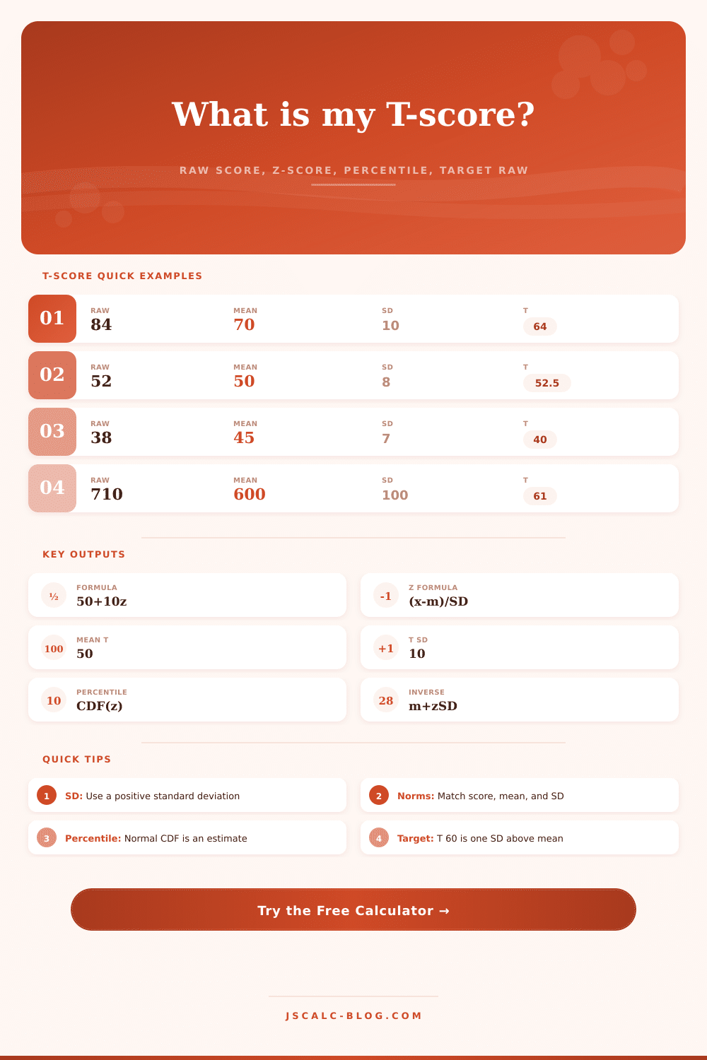
Raw Score: You take a test and get back an eighty-four, thinking it’s pretty good. Then you’re told that class average was seventy with a standard deviation of ten, making the eighty-four look slightly less impressive. Raw scores fail in this way: They are numbers that exist outside of any context, and thus don’t indicate how you stack up against others. By converting your raw performance into a standardized format that allows for easy comparison, T-scores solves this problem.
All you need to do is enter your specific mean and standard deviation into the calculator above, and let it handle all the math (including manual z-score conversion). It is a minor convenience, perhaps, but it eliminates main source of error when understanding standardized tests.
How T-Scores Help Compare Test Results
It’s simple: You take the raw score, subtract the mean, then divide by the standard deviation. That will give you your Z-score, which represents how far from average you are. So if it’s a 1, you’re one standard deviation from average. But z-scores can be messy; decimals, sometimes even negative numbers, and therefore hard for educators and other psychologists to use.
Their solution was multiply the z-score by ten, add fifty, and call it a T-score. That way, you have a number whose average is about fifty and whose standard deviation is ten. This system makes more sense and is simpler to interpret then the z-score itself.
However, what’s key are the inputs, the mean and the standard deviation. Those set the frame of reference. The T-score is only meaningful if you apply it against the correct reference group. And there that’s where many folks trip up. They may be using an adult comparison sample on a pediatric exam, or a local class’ scores as the reference group when they take a nationwide standardized test.
To prevent this mistake the calculator lets you specify a second distribution to compare your score against. Once you have the mean and spread of two distributions, you can compare how one would convert on a different test. It’s just one curve mapped into another. There is nothing magical about it.
In addition, it provides your percentile ranking as well. So, if you have a T-score of sixty, for example, that’s about the eightieth percentile. If it’s a T-score of seventy, then that means you’re in the top two percent. This gives us bands to work with so we don’t get hung up on exact decimal places.
This is why they call them T-scores: each band of ten is a standard deviation. On the page it lays it all out in a reference table which details just what the heck certain T-ranges equate to (e.g., “average,” “high”, etc.). You don’t need to remember those ranges, though, just be aware that each time you increase by ten, you’ve gained another standard deviation of spread.
Of course, there’s an inverse relationship as well which is also helpful because it allows you to reverse-engineer the equation (i.e., given a particular T-score, what was your corresponding raw score?). In other words, if you want to know how many points you need on a test to qualify for something, or set a goal, then you could of plugged in the T-score into the inverse equation. This makes the goal much more concrete.
For example, if you’re applying for a job with a screening process requiring a 60 T-score, you can use this to figure out exactly how many raw points you’ll need to achieve that. You simply do the reverse of the division and subtraction steps; the tool does this for you, but the mental model is straightforward.
The detail lies not only in the T-score itself but also in the spread between those T-scores. A T-score of sixty-five is not the same thing when your distribution is wide as it is when your distribution is narrow. If all the scores cluster tightly, then small deviations matter. But if there’s huge variance, then a given T-score could actualy signify a huge range in raw performance.
That’s why the z-score appears beside the T-score on the calculator. To remind you that what you’re viewing isn’t an absolute measure of ability, but a relative measure of distance. Remember that the number means nothing without context. A high score on a bad test means nothing.
The problem is that it does not evaluate the test itself. It only shows the position of the data within the test, assuming that norms are good and the data is normal. Your responsibility is to feed it information that’s representative of what you’re trying to understand.
If the mean gets jacked up, then the middle is off, meaning the results aren’t accurate. If the standard deviation is bloated, then the T-scores is squashed. But really the reason for standardized scores is that they even things up. Standardized scores remove oddities of each testing form and make it possible to compare one math score from one testing company to a reading score from another. They convert different measurements into like units. The T-Score provides that link across these different measurement systems.
Once you have a T-score, you are no longer concerned about the raw number and can begin to gain some perspective on where you stand in relation to others. And that’s what this all comes down to, fairness. Understanding the score in terms of where you fit in the picture is worthwhile. But entering the parameters is only worthwhile if math does its job. It should free you up to consider what the score indicates in your particular case.