Standard Error of the Mean Calculator
Calculate SEM from sample standard deviation and sample size, then add finite population correction, confidence interval margin, and target sample size planning.
Load a realistic SEM scenario, then adjust any input for your own data.
SEM results
| Confidence setting | Critical value | Margin formula | Common use |
|---|---|---|---|
| 80% two-sided z | 1.282 | 1.282 x SEM | Early screening or rough planning |
| 90% two-sided z | 1.645 | 1.645 x SEM | Exploratory intervals |
| 95% two-sided z | 1.960 | 1.960 x SEM | Most reports and dashboards |
| 98% two-sided z | 2.326 | 2.326 x SEM | Stricter reporting |
| 99% two-sided z | 2.576 | 2.576 x SEM | High confidence summaries |
| Sample fraction n/N | FPC factor | SEM effect | Interpretation |
|---|---|---|---|
| 1% | about 0.995 | tiny change | Usually safe to ignore |
| 5% | about 0.975 | small cut | FPC starts to matter |
| 10% | about 0.949 | moderate cut | Use FPC if N is reliable |
| 25% | about 0.866 | large cut | Limited population precision improves |
| 50% | about 0.707 | major cut | Half the population is sampled |
| Sample size change | SEM multiplier | Margin multiplier | What it means |
|---|---|---|---|
| n doubled | 0.707x | 0.707x | About 29% narrower |
| n tripled | 0.577x | 0.577x | About 42% narrower |
| n quadrupled | 0.500x | 0.500x | Half the SEM and margin |
| n cut in half | 1.414x | 1.414x | About 41% wider |
| n divided by 4 | 2.000x | 2.000x | Double the SEM and margin |
You collect data to find the truth. It comes from the data you collected. It come from the sample mean. The standard error of the mean indicates how much confidence to put in that guess, which is the sample mean. It shows how close your guess is to true population value.
Most folks look at average, then stop there. They don’t bother with the error part; they just report the number. They only give you a point estimate, which are a mistake.
Understanding Standard Error and Sample Size
Once you understand the sample size and standard deviation, simply enter them into calculator above. It’ll do the math on the square root part for you. The hard part is interpreting what these figures mean for your decision based off the data.
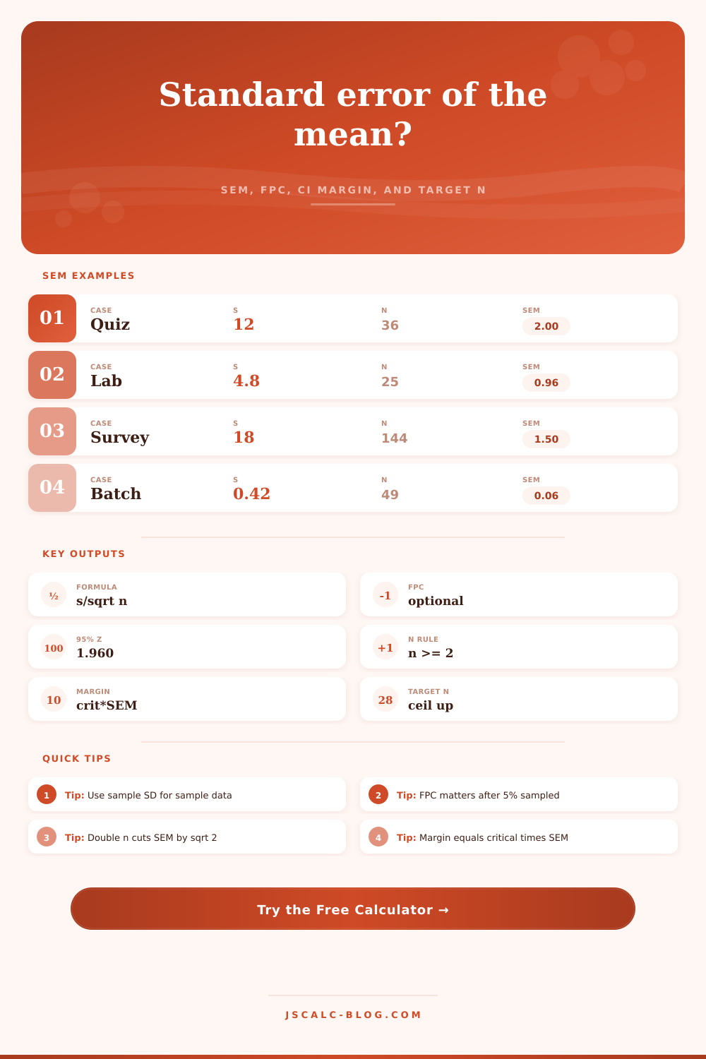
It’s a simple formula: Divide the sample standard deviation by the square root of the sample size. And that’s what drives the whole engine of statistical power: Accuracy scale with the square root of effort. So doubling your sample size doesn’t double your accuracy; in fact, it boost it by only around forty-one percent. To half the error, you need to quadruple the data, which makes many researcher and project manager crazy. We want linear returns on data collection but statistics won’t give us that. It want us to invest exponentially for linear gains.
The tool allows you to toggle between those numbers to visualize the tradeoffs. Add some imaginary respondents and watch the error shrink. This can be a helpful reality check if someone is asking for more budget.
The formula assumes that we’re making guesses about a huge unknown population. The “finite population” correction works when you’re making a guess about something smaller, and you know what the total population size is. Take the example above: We’re auditing a batch of five-hundred units at the factory. Say you pulled a sample of 50, or ten percent of the entire population. That means you’ve narrowed down your knowledge (you’ve replaced some uncertainty) much more then you would by pulling a sample of 50 from an endless sea of items. So the formula recognize that you have less uncertainty to replace here.
It’s good to use it when you know for certain how large the group you’re studying is, since it reduces your error margin. The bigger the percentage of the group you sample, the more relevant it become. If it’s under five percent, don’t bother.
Your interval will be larger but still correct. And if you use it when you shouldn’t, you might get dangerously narrow intervals.
Finally, the confidence interval half-width (also known as the margin of error) is the range around your mean into which you expect true value to fall with some probability. This probability is determined by the confidence level you select. The typical confidence level is 95%, and the corresponding critical value is approximately two, meaning one point nine six is used for precision purposes. Multiply that by your standard error, and you have your margin, the number you present back to the stakeholder as an answer to “how wide should my net be?”. And the answer tells you whether or not you have a tight handle on variable (small margin) or are guessing in the dark (large margin).
One of the nice features here is that the planner allow you to work backwards; if you know how much margin you require, you can figure out size of required sample. In most cases, the answer will be larger than desired.
Standard error is not the same thing as standard deviation (the former is a measure of uncertainty in the mean; the latter is a measure of spread in the data), but this confusion happen frequently. The more variable your population, the more difficult it is to pin down the mean, you’ll need more samples to average out the noise. On the other hand, the less variable your population, the easier the mean is to pin down. So the tool needs standard deviation as input.
You should of calculated that first from your own raw data, or else use it from some other study as a proxy if you don’t have any yourself. That’s a common and acceptable practice in the planning phase. It lets you estimate sample size prior to spending money on collecting new data. That number is rounded up so that you’re guaranteed to hit your precision requirement, and it’s also your target sample size.
What you’ll get isn’t necessarily true; all it guarantees is that you’ll be within a narrower range of possibility. This is what statistics is: measuring uncertainty. It’s not about being certain.
The cost of taking a sample is called the standard error; this is the price you pay for not surveying every person. If you want a smaller standard error, you must take a larger sample. Or, if you don’t mind paying more, you can live with bigger intervals. Your call. But at least the calculator will show you the bill.
You begin with a hunch, and you conclude with an upper limit on that hunch. Actualy, it is moddern way to look at things.