Coefficient of Variation Calculator
Paste one or two datasets to calculate coefficient of variation as CV = standard deviation / mean * 100, with sample or population standard deviation and side-by-side comparison.
📌Data Presets
Load a realistic pair of datasets, then adjust labels, standard deviation type, unit, and rounding.
🔢Dataset Inputs
Calculation Breakdown
🧮CV Method Cards
🗂Sample vs Population Selector Grid
📋Reference Tables
| CV band | Relative spread cue | Typical interpretation | Best next check | Report note |
|---|---|---|---|---|
| 0% to 5% | Very low | Values are tightly clustered relative to the mean. | Confirm measuring resolution is fine enough. | Show extra decimal places if needed. |
| 5% to 10% | Low | Variation is present but usually modest. | Compare with normal tolerance or rubric bands. | Mean and SD usually explain it clearly. |
| 10% to 20% | Moderate | Relative spread may affect ranking or forecasting. | Look for outliers and subgroup patterns. | Include n and the SD type. |
| 20% to 40% | High | Values vary widely compared with their mean. | Review whether one data source is mixed. | Use a chart or contribution table. |
| 40%+ | Very high | Average alone may be misleading. | Inspect distribution shape and scale limits. | Pair CV with median or range. |
| Mean near 0 | Unstable | CV becomes undefined or misleading. | Use SD, MAD, or range instead. | Do not force a CV percentage. |
| Profile | Good CV use | Caution | Common unit | Useful companion stat |
|---|---|---|---|---|
| Education scores | Compare score consistency across sections. | Bounded 0 to 100 scales limit spread. | points | class mean |
| Quality control | Compare precision across part sizes. | Small CV can still fail tight tolerances. | mm, g | range |
| Survey ratings | Compare relative response variation. | Ordinal scales are not true ratios. | stars | median |
| Operations counts | Compare workload variability by team. | Seasonal cycles can inflate CV. | orders | percentile |
| Lab measurements | Check repeatability and instrument noise. | Near-zero means make CV unstable. | mg/L | resolution |
| Timing data | Compare relative process consistency. | Right-tail delays can dominate SD. | seconds | p95 |
| Financial ratios | Compare return variability to average return. | Negative or tiny means need care. | percent | drawdown |
| Growth measurements | Compare consistency across growth groups. | Check whether starting sizes differ. | cm, g | growth rate |
| Dataset | n | Mean | SD | CV | Min to max | Contribution cue |
|---|---|---|---|---|---|---|
| Dataset A | 8 | 84.25 | 4.01 | 4.76% | 78 to 91 | Calculate to refresh. |
| Dataset B | 8 | 41.38 | 3.84 | 9.29% | 35 to 47 | Calculate to refresh. |
💡Coefficient of Variation Tips
Two datasets has similar standard deviations, yet one is relatively stable and the other is chaotic. Dispersion metrics in raw form let you down. They don’t account for scale. That’s where coefficient of variation comes in.
It measures variability in terms of a percent of the mean. It converts absolute spread to relative risk. You can now measure a stock price of $10 and a stock price of $500 on the same plane, otherwise you’re comparing apples to oranges (and doing so wrong).
Why Use Coefficient of Variation
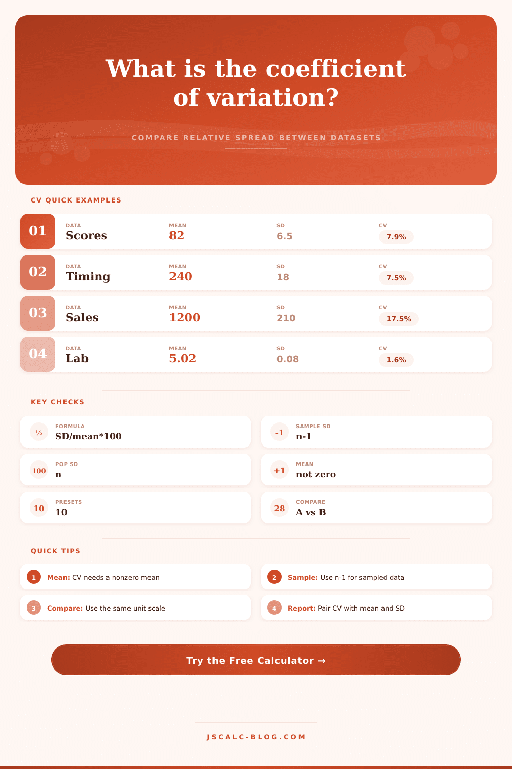
The formula is to divide standard deviation by the mean then multiply by one hundred. That’s what the calculator does for you. Half of the problem is getting that number. The other part is determining the correct denominator when calculating the standard deviation.
When your data set are a sample from a greater population, you want to calculate using the sample standard deviation. This formula use n, 1 as the divisor. Why? It adjusts for bias when trying to estimate parameters. Using the population equation on a data set is like looking at the world through rose-colored glasses. Your data appears smoother than it realy is. Guess where this hurts you? In your risk assessment.
How do you choose between types of standard deviations? That depends off context. If you have all the points, then you want population standard deviation. If you’re using the entire day’s output from a factory line, then you’ve got it. You’re measuring the entire thing, you’re not approximating it.
Unfortunately, most folks defaults to the sample standard deviation because that’s what they always use. It is no problem if you just want an approximation, but it is sloppy otherwise. Toggle this setting in tool. Now you’ll be forced to consider where your data came from. Don’t fool yourself into thinking that a convenient sample are a full census. The metric respects its boundaries.
If the mean is negative or zero, the coefficient of variation becomes meaningless (the denominator divides by zero). If the denominator equals zero, dividing makes no sense at all (undefined). If the mean is negative, you flip the meaning of variance when you divide by a negative number. These restrictions make the coefficient suitable only for ratio scale data.
Ratio scale data are represented with a true lack of something at zero. Examples include monetary values, times, and weights. Avoid using it for temperature measured in Fahrenheit or Celsius because the zero here isn’t true zero; it’s an arbitrary point.
The calculator will warn you as your average nears zero. Why? It saves you from publishing a nonsense percentage.
The higher the coefficient, the greater the relative variability between two group. Even if one group’s standard deviation is bigger than another group’s, the higher coefficient will still hold. This is unintuitive, which is why we need the coefficient in quality control and finance.
High consistency means a low coefficient. That’s what you want to see when measuring manufacturing tolerances. Does high variance mean high growth? Maybe that’s what you should of seen from high-growth startups.
Here’s the reference table. It gives you bands of interpretation. It allows you to label a 10% variation as either: (a) Alarming! Or (b) Acceptable!
Low variation in surgical outcomes? You want that. Low variation in your company’s ideas? Stagnation?
There’s a side-by-side comparison feature, which comes in handy if you’re trying to A/B test something. You get the percentage point difference right there, so you know how much bigger the result was on one side different than the other. It’s a little thing, but when it comes time to justify making a change to a process, that kind of detail helps. Managers are a skeptical bunch and they don’t just want to see the scores; they want to see the change.
A coefficient of variation isn’t truth; it’s a lens. When you zoom out from the individual data point, you see the distribution’s shape compared to its center. Compare different scales. Combine it with the raw standard deviation and mean for full context. The absolute spread might be huge even with a low coefficient, provided that the mean is enormous. A high coefficient may be manageable if the stakes aren’t high. Trust the percentage, but verify the reality behind it. Use raw numbers to make reliable decisions.