Pooled Standard Deviation Calculator
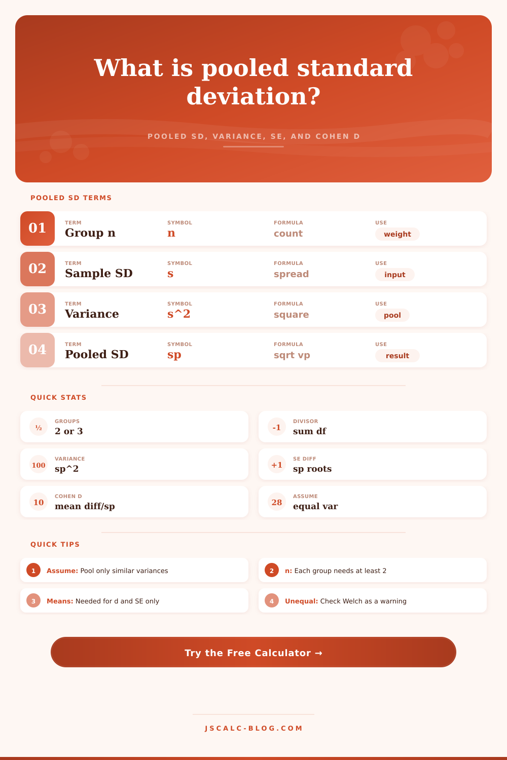
Combine two or three group sample standard deviations into one pooled SD, then calculate pooled variance, standard error for a mean difference, and Cohen d under the equal variance assumption.
Two-group mode also shows the standard error for the difference and Cohen d.
Pooled SD is most appropriate when group spreads are plausibly similar.
Group 3 pairs are used only when three-group mode is active.
Controls displayed pooled SD, variance, SE, and effect size.
Group 1
Group 2
Group 3
| Group | n | Mean | Sample SD | Variance s2 | df = n - 1 | df x s2 |
|---|---|---|---|---|---|---|
| Enter group statistics above to calculate contributions. | ||||||
| Pair | Mean difference | Pooled SE | t using pooled SE | Cohen d | Magnitude cue |
|---|---|---|---|---|---|
| Pairwise effect results appear after calculation. | |||||
| Check | Your value | Common cue | Interpretation | Next calculation |
|---|---|---|---|---|
| Variance assumption diagnostics appear after calculation. | ||||
| Use case | Groups | Inputs needed | Assumption | Main output | Do not use when |
|---|---|---|---|---|---|
| Independent t test | 2 | n, mean, SD | equal variance | SE and t | variances very different |
| Cohen d | 2 | means and SDs | similar spread | standardized difference | ordinal-only scales |
| ANOVA planning | 3+ | n and SD | within-group variance | common SD | heteroscedastic groups |
| Lab repeatability | 2 or 3 | n and SD | same method spread | pooled variance | different instruments |
| Meta summary | 2 or 3 | summary stats | same outcome scale | pooled SD | different units |
| Welch comparison | 2 | n, mean, SD | unequal variance | Welch SE | using pooled d alone |
You’ve got two sets of data in your spreadsheet. One group has taken new medication; another group has taken a placebo. The average outcome is different, but was it because the new drug worked? Or did you just see some random variation? To figure out the answer, you’d like to know: How widely do the data points fluctuate around their mean?
Taking an average of the two standard deviations won’t cut it. You’re likely to wind up with wrong answer, partcularly when your sample sizes aren’t equal. That’s where pooling comes into play. It calculates a single, weighted measure of spread that accounts for the contribution from both group.
When to Use Pooled Standard Deviation
But it’s easy to misunderstand: It’s really quite a simple concept. It’s a weighted average of variances, with weights being degrees of freedom. That’s just jargon; what does that mean in English? Well, bigger groups carry more weight in the overall result compared too smaller groups. And why wouldn’t they? If we calculate standard deviation based off 50 people, it’s going to be more reliable than if we calculate a standard deviation based on five.
The calculator above takes care of that weighting for you, you don’t need to go back and multiply each variance by (N-1), where N is the sample size. Just input your existing summary stats.
People often do this without verifying whether their assumption of equal variance is justified. The equal-variance (aka pooled) method also makes an assumption that variability within each group is approximately similar. But what happens when one group is tightly clustered and the other scatters wildly? Pooling those two groups will distort the answer. It hides the variation, this is where people go astray. They use the pool only sometimes, but they always treat it as a regular step in the process.
Always look at the ratio of larger standard deviation to the smaller standard deviation. If that ratio is approaching two or greater, then maybe you’re best-served by a Welch’s test, which doesn’t assume that the variance are equal. For this reason, the tool gives you a diagnostic cue: the largest SD divided by the smallest SD. If this number is small, then you can safely pool. If it’s large, the tool will let you know. It will prevent you from falling into trap of believing that your pooled standard error is anything other than a misleading quantity.
After all, the pooled figure is what the whole thing hinges upon; the standard error for the mean difference relies completely on it. So when your pooled SD is way off, your confidence intervals end up being either too wide or too narrow. This causes you to wrongly accept or reject null hypothesis. This denominator is also central to Cohen’s d, another output provided by the tool. In standardized units, it describes how big difference between two group is. Cohen suggested that an effect size of d = 0.8 is generally large, but that’s only true if the denominator represent the natural variation in that population. If instead you’ve pooled variance across groups with inherently different levels of variation, then your effect size represents some sort of hybrid measure. It doesn’t cleanly map to any existing benchmark. It is a small thing, but it matters for reproducibility.
So why do we average the squares of standard deviations? Because the standard deviation doesn’t add the same way variance does. Variances are the expected squared deviation from the mean. And when you add up multiple groups, you are adding up their sums of squared error. In order to get back into original units, you have to go through the variance domain first with the math. Add up the squared errors, divide by total degrees of freedom, and finally take the square root back out. That maintains the necessary statistical properties for inference. If you skip over the squaring, you break those properties.
That calculation shows up everywhere from software engineering A/B tests to clinical trials in practice. You’re running a clinical trial to see whether your drug actualy lowers someone’s blood pressure significantly. Or maybe you’re doing an A/B test to see if different colored button leads people to click more. Either way, you need some idea of what the background noise looks like. Underestimate it and you’ll think you’ve discovered something when you haven’t (there is no signal). Overestimate it and you might miss actual improvements. When the assumption holds, pooling provides you with best estimate of that background noise.
This is where it gets powerful: the beauty of this method is how efficiently it squeezes juice from your data. By assuming that both the population itself and our measurement process have some variance, this method shows that the variance isn’t just a characteristic of one sample, but of several. If we’re taking multiple groups from the same or similar populations, each group’s own variance is an imperfect estimate of the true population variance. But together they form more stable estimate. They smooth out the random nature of small-sample results.
At the end of the day, statistics are all about striking a balance between being practical and rigorous. Sometimes you don’t have time to check each assumption perfectly. But you can train yourself to question the inputs. Examine your standard deviations. How do they compare? Are your sample sizes wildly different? If so, then you’ll know to take a cautious approach. If they are similar, then there’s a clean, defensible way forward: pool them, and use tools at hand to account for it. They allow you to turn a bunch of different, noisy data into one useful number where you can finally see the signal.