Standard Deviation of Population Calculator

Standard Deviation of a Population Calculator

Enter a complete data set and this tool returns the population standard deviation sigma, the population variance sigma squared, the population mean mu, and the sum of squared deviations, dividing by N rather than n minus 1. It also lists each z-score and checks how well your data follows the empirical 68-95-99.7 rule.

🎯Full Population Presets

📊Your Population Data

Population data set (every member of the group)

Paste the whole population. Separate numbers with commas, spaces, or new lines. Because this is a full population, the divisor is N.

Decimal places on results

Controls rounding on sigma, variance, mean, and every table.

Sort values before display

Sorting reorders the deviation table only; it never changes sigma.

Show per-value z-scores

The z-score tells how many sigma each value sits from the mean.

Show squared-deviation steps

Reveals how each (x - mu) squared adds up to the sum of squares.

Empirical rule comparison

Counts how many values land within 1, 2, and 3 sigma of mu.

Report sigma as percent of mean

Sigma divided by mu, times 100, shows relative spread.

Population Std Dev sigma 0 square root of the variance

Population Variance sigma^2 0 sum of squares divided by N

Population Mean mu 0 sum of all values over N

Sum of Squared Deviations 0 across N = 0 values

Per-Value z-scores

Value x	x - mu	z = (x - mu) / sigma	Within

🔢Formula Snapshot

muSum x / N

sigma^2SS / N

sigmasqrt(SS / N)

z(x - mu) / sigma

⚖Population vs Sample Formula

Step	Population (this tool)	Sample Estimate	Why It Differs
Center	Mean mu = Sum x / N	Mean x-bar = Sum x / n	Same arithmetic mean
Deviations	x minus mu	x minus x-bar	Distance from the center
Sum of squares	SS = Sum(x - mu)^2	SS = Sum(x - x-bar)^2	Identical squaring step
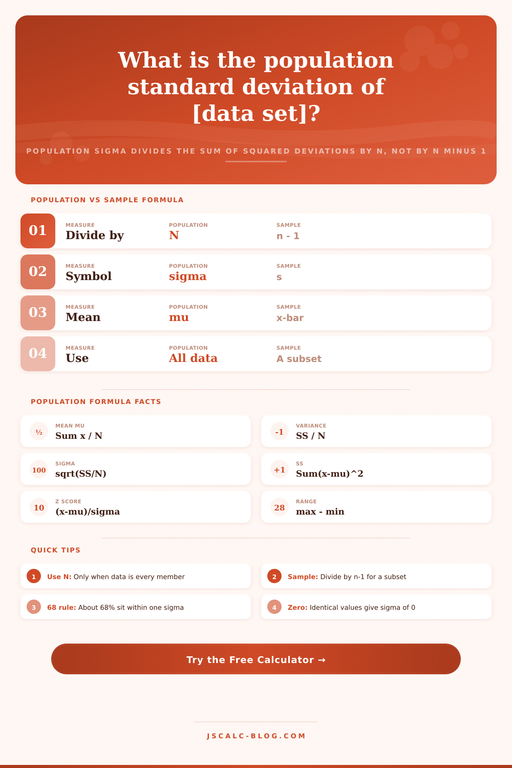
Divisor	Divide by N	Divide by n minus 1	Bessel correction for samples
Variance	sigma^2 = SS / N	s^2 = SS / (n - 1)	Sample value is larger
Std deviation	sigma = sqrt(SS / N)	s = sqrt(SS / (n - 1))	Sample s exceeds sigma
Meaning	Exact spread of all data	Unbiased estimate of sigma	Depends on data scope

📋Live Squared-Deviation Table

Value x	Deviation x - mu	Squared (x - mu)^2
N = 0	Sum of deviations = 0	SS = 0

🎳Empirical Rule Bands (Your Data)

Band	Range mu ± k sigma	Expected % (Normal)	Actual % (Your Data)
Within 1 sigma	mu ± 1 sigma	68.27%	0%
Within 2 sigma	mu ± 2 sigma	95.45%	0%
Within 3 sigma	mu ± 3 sigma	99.73%	0%

📏Example Populations Comparison Grid

Population	N	Mean mu	Sigma	Variance	Range
Class of 30 scores	30	80.30	8.19	67.14	31
All employee ages	12	38.75	9.29	86.35	29
Every machine part mm	10	25.02	0.05	0.0026	0.15
Full season rainfall	12	3.29	1.42	2.01	4.60
Complete survey n=20	20	6.35	2.06	4.23	7
All 12 monthly sales	12	47.83	13.16	173.14	44
Whole batch weights	10	500.90	3.15	9.89	10
Census block ages	15	34.87	21.42	458.78	68
All test runs	10	101.60	4.13	17.04	13
Team salaries	8	72.50	14.79	218.75	42

⚙Formula Breakdown

Count NN is how many values are in the whole population. Because you enter every member, N is the divisor everywhere, not n minus 1.

Population mean mu = Sum x / NAdd every value and divide by N. For 82, 76, 91 with N = 3 the mean is 249 / 3 = 83.

Deviation x − muSubtract the mean from each value to see how far above or below center it sits. Deviations always sum to zero.

Sum of squares SS = Sum(x − mu)^2Square each deviation so negatives do not cancel, then add them. This SS is the raw spread of the data.

Population variance sigma^2 = SS / NDivide the sum of squares by N to get the average squared deviation. This is the population variance.

Population sigma = sqrt(sigma^2)Take the square root of the variance to return to the original units. This is the population standard deviation.

z-score z = (x − mu) / sigmaEach z-score counts how many standard deviations a value lies from the mean, positive above and negative below.

CV = sigma / mu × 100The coefficient of variation expresses sigma as a percent of the mean, useful for comparing spread across different scales.

💡Population Sigma Tips

Only use N for a true population: Divide the sum of squares by N solely when your data includes every member of the group, such as all 30 students in one class or every part in a finished batch. If your numbers are just a sample drawn from a larger group, use the sample formula that divides by n minus 1 instead. That Bessel correction gives an unbiased estimate of the unknown population sigma and always returns a slightly larger value than the population formula on the same numbers.

Read spread with the empirical rule: For data that is roughly bell shaped, about 68% of values fall within one sigma of the mean, about 95% within two sigma, and about 99.7% within three sigma. Turn on the empirical comparison to see how your actual counts stack up against those targets. A close match suggests near-normal data, while a big gap hints at skew, outliers, or a distribution that is not bell shaped, so read sigma with that context in mind.

This page’s standard deviation of a population calculator is a measure of just how closely (or loosely) all members of a set of number cluster to their average. When you have all the people in a group, you use population formula. That could be the whole class, the entire batch, or every month of a finished year.

It uses the approach: divide the sum of squared deviations by N. In practice, that means tool will go through your data set to work out the population mean mu. It will calculate the sum of squared deviations, the variance sigma squared, and the standard deviation sigma. Then it will check how well the spread matches the classic empirical rule.

How This Calculator Works

When it comes to standard deviation, it’s answering one quick question: how far from the middle are the numbers on average? If their sigma is tiny, they’re clumped around the mean. If their sigmas is big, then they’re spread far and wide.

Here’s the catch: the qualifier population matters. This isn’t some sample we pulled from a larger set; this IS the thing whose numbers you want to know about. You have all of them, so you don’t need to account for the fact that you might be off because of your sampling method. Your denominator is just N, aka number of observations.

The math runs in a fixed order. It adds all values and divides by N to get the population mean (mu). Then it computes each deviation, i.e., the value minus mu. So it tells you how far each point is from the mean, above or below. It doesn’t let those plus and minus gaps cancel; instead it squares them. That gives you sum of squared deviations. Divide that by N and that’s the population variance. And take the square root of the variance and you have sigma back again in the same units.

That’s where some people get confused. If you have a whole group (i.e., all the numbers), then dividing by N does indeed give you correct spread of those numbers. If you have a sample and are trying to estimate the true spread in an unknown larger population, then we uses n, 1 as the divisor. This is just the statistician’s way of accounting for the fact that a sample will tend to under-estimate the actual spread in the larger population. So you’ll always see that the sample standard deviation is slightly bigger different than the actual population value calculated from the same numbers.

Four central results cards populate every calculation. First: the population standard deviation sigma. It can also appear as the coefficient of variation, which is sigma as a percent of the mean. Second: variance, the square of sigma. Third: the population mean mu, or the balance point of your data. Fourth: N and the sum of squared deviations; these are the raw ingredients that feed sigma and variance.

To help visualize this, you can activate the per-value z-scores option, which plots the value’s location relative to its mean. If your score is equal to the mean, it has a z-score of zero. One full standard deviation above (or below) is +1 (-1). Two standard deviations below is -2. Each value becomes placed onto a consistent scale through z-scores. You can use this to highlight values that are unusually low/high. Anything with a z greater than ~3 is worth considering as an outlier.

The empirical rule describes the kind of pattern you can expect to see for roughly normal data. At one sigma, approximately 68 percent of the values should be inside this range. At two sigma, approximately 95 percent of the values should be inside this range. At three sigma, approximately 99.7 percent of the values should be inside this range. The number of your own values that end up in each band gets counted by the calculator. It displays both the expected and observed percentages. A close match between the two columns means your data follows a normal distribution. Difference suggests outliers or skewing.

Each of these loads a whole set of data for typical life situations… All the parts on a machine in millimeters, all the employees’ ages, a class of 30 score, etc. There are other presets for batch weights, team salaries, census block ages, a full survey, a full season’s worth of rainfall, monthly sales, and test runs. These represent a full population… Which is just what the divide by N formula is for. Now you see how other sets of real data spread out, and tool recalculates instantly so you can compare them.

When a data set exceeds a few values, computing its population standard deviation manually becomes tedious. You’re prone to using the incorrect divisor. This calculator eliminates the arithmetic drudgery and formula confusion by parsing through your entire population, dividing by N, and displaying all of the relevant metrics in a single screen. Paste in a complete dataset or load one of our presets. If desired, tinker with the options to display the working steps. Read the tables and cards. Within seconds, the population standard deviation calculator returns reliable numbers. It transforms raw data into a clear picture of spread.

Actualy, you should of used it sooner. All the furnitures in my house could use this kind of math. If we want to see how the moddern age affects things, we can find out by using this tool for our calculation. We would of known the result if we had looked closer. It is naturaly easy to use.