Skewness Calculator
Paste numeric values in this JSCalc-Blog.com calculator to calculate adjusted Fisher-Pearson skewness G1, population moment skewness, central moments, tail direction, and value-level contributions.
🎯Data Presets
Load a real distribution shape, then adjust the method, label, unit, and table depth.
🔢Dataset Inputs
Calculation Breakdown
📌Current Distribution Grid
📈Shape Reference Grid
📋Reference Tables
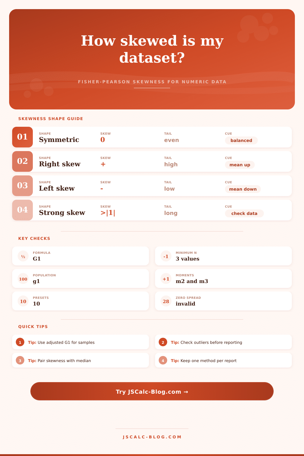
| Skewness range | Shape label | Tail cue | Typical reading | Best next check |
|---|---|---|---|---|
| -0.10 to 0.10 | Nearly symmetric | Balanced tails | Mean and median usually tell a similar story. | Report spread and center. |
| 0.10 to 0.50 | Slight right skew | Longer high tail | A few high values pull the average upward. | Compare mean with median. |
| -0.50 to -0.10 | Slight left skew | Longer low tail | A few low values pull the average downward. | Check floor effects or penalties. |
| 0.50 to 1.00 | Moderate right skew | Visible high tail | Median may be a better typical-value summary. | Inspect top contributors. |
| -1.00 to -0.50 | Moderate left skew | Visible low tail | Lower-tail values may dominate the cubic moment. | Inspect bottom contributors. |
| Above 1 or below -1 | Strong skew | Dominant tail | Distribution is asymmetric enough to require context. | Check outliers or mixed populations. |
| Method | Formula | Minimum n | Best use | Important note |
|---|---|---|---|---|
| Adjusted Fisher-Pearson G1 | sqrt(n(n - 1)) / (n - 2) * m3 / m2^(3/2) | 3 | Sample datasets and statistical summaries. | Applies a finite-sample adjustment to moment skewness. |
| Population moment g1 | m3 / m2^(3/2) | 2 | Complete population values or descriptive dashboards. | No sample correction is applied. |
| Second central moment m2 | sum((x - mean)^2) / n | 2 | Denominator of skewness. | Must be greater than zero. |
| Third central moment m3 | sum((x - mean)^3) / n | 3 | Direction and strength of asymmetry. | Positive values indicate right-tail pull. |
| Mean minus median | mean - median | 1 | Quick direction cross-check. | Useful but not a substitute for G1. |
| Contribution table | (x - mean)^3 | 3 | Finding tail-driving values. | Cubic terms make extremes stand out. |
| Rank | Value | Deviation | Squared deviation | Cubed deviation | Contribution cue |
|---|---|---|---|---|---|
| -- | -- | -- | -- | -- | Calculate to refresh. |
💡Skewness Tips
The old saying goes that numbers like averages can be misleading, which isn’t entirely accurate. Averages is simply poor storytellers. They present you with a point of reference, a center of gravity in your data set, without showing you the shape of the tale. This is where skewness come into play. It is a measure of asymmetry. It is the reason why your average income might feel less truthful than your median income. It also explains how an extreme value or two can pull an entire data set off balance.
Once you grasp this, you’re able to move beyond flat number and into distribution itself. So, we’ve built a calculator that does all the complicated moment calculations for you. Simply copy and paste in your numbers (server latency logs, delivery times, exam scores) and let the tool break them down for you.
Why Skewness Is Important
One thing to keep in mind very early on: Is this population data or a sample? In other words, do you have all of the data points for the set you’re interested in, or just some of it? If the latter; if you’re examining only a subset of something bigger, you’ll want adjusted Fisher-Pearson G1. Because it takes into account a correction factor, it tend to not overstate skewness in small samples. If you have all data for what you’re after, though, then you’ll want the population moment skewness. Again, it’s a little bit of a technical detail, but an important one for getting accurate results.
If you plug some numbers into tool, what does it do? It computes third central moment, which means it cubes the differences from average. Cubing is aggressive. A single outlier can dominate the results and its effects are amplified much more further than if we squared the deviations. This is where people go wrong. They think skewness is only about direction of tail, but it’s really about how heavy tail is.
If there are too many high values then they stretch out the distribution, pull up the mean relative to median, creating a right skew. Conversely, if there are too many low values then they drag down on the mean, creating a left skew. It’s all pretty easy ranges laid out in the reference table at top of page which helps you make sense of what it is you’re looking at. A score around zero indicates that your data is symmetric, a normal bell curve. In real world this is uncommon.
Data is often messy. Reaction times, income, house prices isn’t normally symmetric. There’s an open end and a bounded end. You can’t have negative time or negative income. So the tail must run off in opposite direction. A natural limit on the value naturaly introduces a skewed distribution with a predictable shape. Skew that is particularly strong, typically above +1 or below -1, is flagged by tool as something to pay attention to, suggesting that you look for potentially mixed populations or outliers in your data.
But why should we care about this test? Standard statistical tests usually rely on the assumption that your data follow a normal distribution. When it’s really skewed (i.e., heavy-tailed), these tests will screw up and provide you with false confidence in your results. The part of the results section I like best is the contribution table, which reveals to you exactly what values are pulling out the skew. Maybe there are two or three outlier observation that account for all the asymmetry. If so, then you shouldn’t be thinking of the skew as something inherent in the group, just something resulting from some odd observations.
But skewness isn’t so much an answer as it is a way to ask a better question. When does the mean mislead? What’s the typical experience, if a few outlying extreme examples hide what is typical? And then after understanding its shape, what do you do next? Trim off the outliers? Use median instead? Maybe transform the data in some other way? You should of looked at it first.
The numbers come from the calculator. But the insight, the connection between the numbers and reality of your actualy data set; that’s up to you.