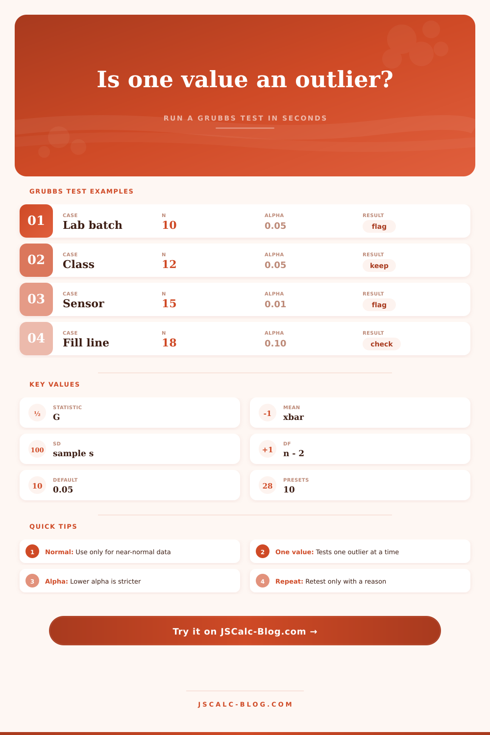
Grubbs Test Calculator
Paste a dataset to test whether the most extreme value is a single outlier using G = max |x - mean| / s and the Grubbs critical value based on alpha, n, and t degrees of freedom.
📌Data Presets
Load a realistic dataset, then adjust alpha, label, units, rounding, and whether to display signed or absolute deviations.
🧮Calculator Inputs
Calculation Breakdown
🗂Test Setup Grid
📋Reference Tables
| Step | Quantity | Formula | Calculator output | Reason for the step |
|---|---|---|---|---|
| 1 | Mean | sum(x) / n | -- | Center point for deviations. |
| 2 | Sample SD | sqrt(sum((x - mean)^2) / (n - 1)) | -- | Grubbs uses sample standard deviation. |
| 3 | G statistic | max |x - mean| / s | -- | Standardizes the biggest departure. |
| 4 | Critical t | t at 1 - alpha / (2n), df = n - 2 | -- | Controls the two-sided single-outlier test. |
| 5 | Critical G | ((n - 1) / sqrt(n)) * sqrt(t^2 / (n - 2 + t^2)) | -- | Reject if G is greater than critical G. |
| Rank | Input position | Value | Signed deviation | Absolute deviation | Individual G | Candidate note |
|---|---|---|---|---|---|---|
| Calculate to refresh the deviation table. | ||||||
| Alpha | Meaning | Typical use | Effect on critical G | Practical note |
|---|---|---|---|---|
| 0.10 | 90% confidence screen | Exploratory cleanup | Lowest listed threshold | More likely to flag a value. |
| 0.05 | 95% confidence screen | Common default | Middle threshold | Good first-pass setting. |
| 0.025 | 97.5% confidence screen | Stricter QA | Higher threshold | Needs stronger evidence. |
| 0.01 | 99% confidence screen | High-stakes review | Highest listed threshold | Flags only very extreme values. |
🔢Alpha / df Critical G Table
This grid is generated from the same critical formula used by the calculator for the current sample size neighborhood.
💡Grubbs Test Tips
The thing about outliers is you have nine values that appear completely typical, then there’s one that doesn’t even come close. Maybe that’s not an error; maybe it isn’t. But since it’s so far away from the cluster, you wonder if something is amiss. Should you include it? Suspect it? Throw it out? Daily, statisticians asks themselves just that. Intuition often fails. Without some sort of framework, the human brain can’t determine what’s statistically significant.
Now we introduce the Grubbs test. Why is the Grubbs test helpful? It eliminates guessing. It takes lone extreme value and tests it against the mathematically expected patterns for a normal distribution. It’s pretty straightforward: grab the value farthest away from the mean (high or low) and then measure how many standard deviations it is away. Divide that most extreme value by the standard deviation of your sample to get the G statistic, which the calculator provides for you. Then compare that against a critical threshold; if it’s above the critical threshold, mark the point as an outlier.
How to Use the Grubbs Test
But what’s that threshold? That vary depending on your sample size and how stringent you wish to make your test. Small samples inherently have more noise in them than large ones, so we need a bigger deviation before marking something as an outlier. And that’s exactly what the tool takes into account, with t-distribution degrees of freedom. So regardless of whether you have ten points or fifty points, the test is fair.
This is where the rubber hits the road: Which significance level (also known as “alpha”) will you use? For most purposes, 95% confidence, that’s alpha = 0.05, is a good default. That’s what most of us keep using. If you’re working on something really important, such as aerospace engineering or pharmaceutical manufacturing, you may increase this threshold to 99%, or even 99.9%. (That’s alpha = 0.01.) On the other hand, perhaps you’re poking around in some noisy data set and need to clean it up so you can plot it. In that case you could loosen things up to alpha = 0.10 or above. That means you have to have overwhelmingly strong evidence against including a certain data point before you toss it out.
The table below shows the change in thresholds based off different values of alpha. You can see directly how your decision impacts the result.
First, let’s talk about how not to use the Grubbs test. It’s designed to identify a single outlier. It will not give you more than that in one go. Removing a flagged point and running it again on the smaller data set won’t find the next-worst offender. It also won’t have anything to base its decisions on. Think of what happens when you remove a point: you change the data set. In this case, each point has been assumed approximately normal. By peeling them off one at a time you invalidate the data with every peel. Now sure, it’ll run the numbers. But it doesn’t know whether or not you’re being reasonable; it doesn’t know about the methodology.
If your domain knowledge tells you there should only be one bad point (or two!), then maybe there really is a justification for doing another test. The calculator shouldn’t dictate that; it’s up to you. Take a sensor. It spikes for some known electrical interference. This is a valid reason to exclude it. Take an assay run by a lab tech who reads one off. The reagent batch was old. Valid reason to investigate, maybe even exclude that read. But take out a point just because it screws up your regression line? That is statistical cherry picking.
You get the p-value, you get the G value from the calculator. Your knowledge of the process provides context. In particular, that’s where the tool’s deviation table helps. It lists all the points according to how far away they are from the average. Occasionally the second-most-extreme point will be only very slightly less extreme than the first. The test might catch one but not the other, and it seems arbitrary. Not at all! It’s an expression of how likely each outcome is. If a point really is distant, it matters.
In the end though, outlier detection isn’t so much about the math as it is about the story the data want to share with us. The Grubbs test is the proof, providing the mathematical evidence to back up what you think might be true. In other words, does that one oddball number represent bad luck or is there potentially something bigger at play?
By the time you input the numbers into the calculator, you aren’t left only knowing whether to cast it aside or not. Instead, you’re left with a method for defending your data decision-making. Keep it or cast it aside, but either way, you’ll have a solid reason for doing so. And that’s where the beauty of the tool lies: turning a hunch into a defensible conclusion.
You should of checked the data first. It would of been easier.