Modified Z-Score Outlier Calculator
Enter a numeric dataset to calculate median, MAD, modified z-scores, common outlier flags using abs(modified z) > 3.5, zero-MAD handling, and robust versus ordinary z-score behavior.
Load a realistic dataset, then adjust the outlier threshold, zero-MAD rule, standard z-score comparison, row display, label, and unit.
Enter at least three values to flag robust outliers.
| Input # | Value | Distance from median | Modified z | Ordinary z | Flag result |
|---|---|---|---|---|---|
| Enter values to see robust outlier flags. | |||||
| Step | Formula | Purpose | Current value |
|---|---|---|---|
| Calculate to fill method steps. | |||
| Scenario | Median | MAD | Mean | Sample SD | Modified z flags | z-score flags |
|---|---|---|---|---|---|---|
| Calculate to compare robust and ordinary flags. | ||||||
| Rule | Typical cutoff | Best used for | Watch out for |
|---|---|---|---|
| Modified z-score | abs(score) > 3.5 | Skewed or outlier-prone numeric data. | MAD = 0 needs explicit handling. |
| Ordinary z-score | abs(score) > 3 | Roughly bell-shaped data with stable mean and SD. | Mean and SD move when extremes are present. |
| IQR fences | Q1 - 1.5 x IQR, Q3 + 1.5 x IQR | Boxplot-style quick flagging. | Can flag many points in heavy-tailed samples. |
| Strict zero MAD | undefined | Reports that modified z cannot be computed. | No ranking among non-median values. |
| Unequal zero MAD | x not equal to median | Flat data where any deviation is noteworthy. | May be too sensitive for rounded data. |
| IQR backup scale | MAD substitute = IQR / 1.349 | Fallback when IQR still has spread. | It is no longer a pure MAD calculation. |
There’s a way for you to use statistics to find outliers in your data: it’s called the modified z-score. It resolves the push-pull of suspicion versus curiosity we feel when something doesn’t look right.
If you have perfectly symmetrical data (e.g. Following a textbook bell curve), standard z-score is fine. But this isn’t how things play out in the real world. Extreme values pulls the mean towards themselves, shrinking the standard deviation in the process. This causes all the other points to appear more normal then they are.
What is the Modified Z-Score?
The fix? Don’t let outliers determine the rules by which they’re detected. The modified z-score fixes this issue using median instead of mean and the median absolute deviation (instead of the standard deviation). Why? Because median does not depend on position: it anchors the center point of data no matter where the tails extend.
Once you’ve entered your data into the calculator on the page, it will take care of the math for you. That way you can concentrate on what these results tell you about your research or quality control process. Enter raw numbers and the tool calculates a reliable z-score for every point which indicates how many units away that point is based off the center in terms of typical spread. In other words, it’s a cleaner way to separate the signal from the noise. The points you’re looking for don’t hijack mean.
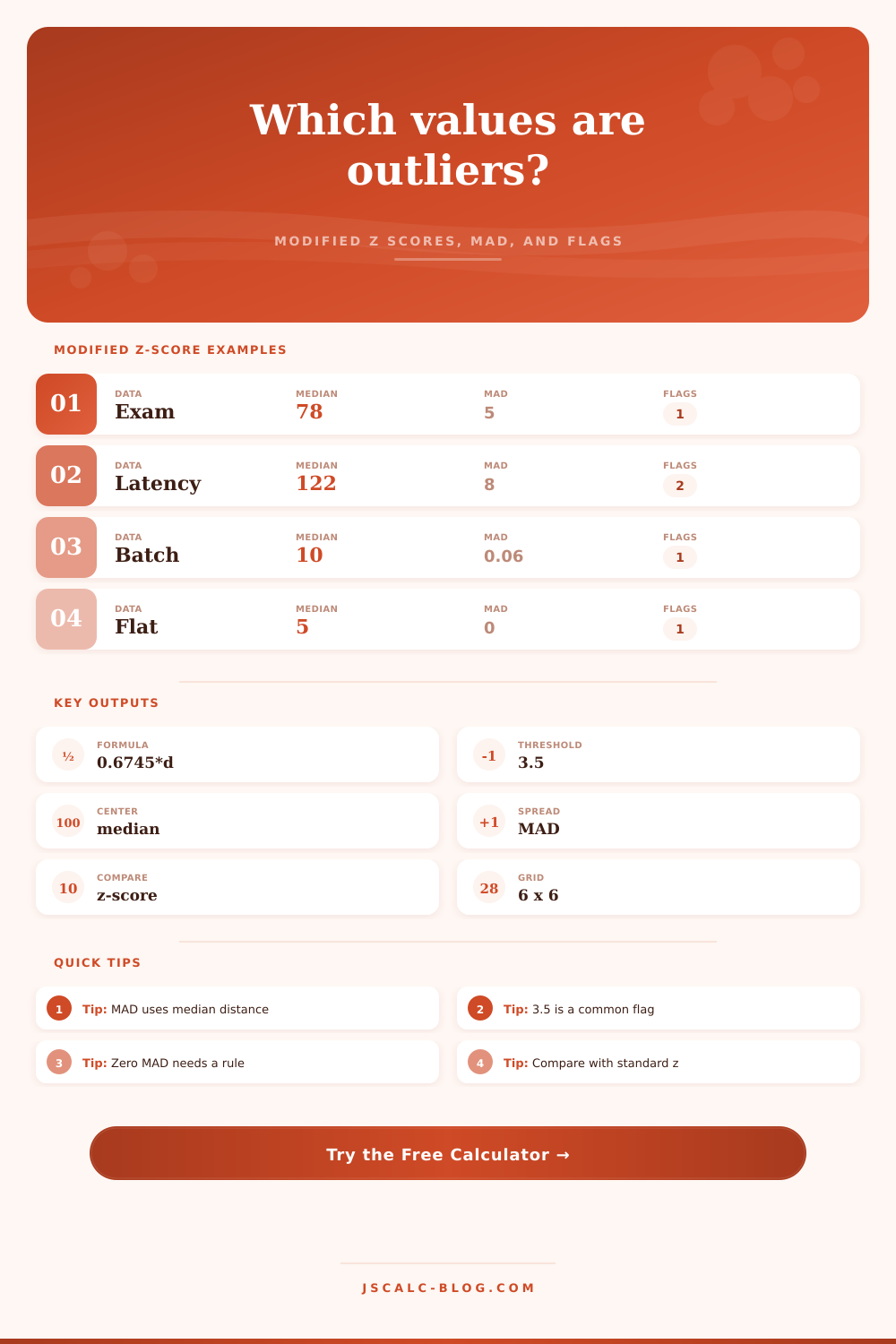
Typically, we use a modified z-score with a threshold value of 3.5. Why do we do that? Why aren’t we using common threshold of 3 for ordinary z-scores? We do this because the median is stable. Unlike standard deviation and mean, the median and MAD are resistant to outliers. So when we look at the distribution of our scores, they’re not going to behave like normal distribution that the standard approach assumes. We would of end up calling too many normal scores anomalies if we used a threshold of 3. To make up for more tightly clustered robust scores, we apply a 3.5 threshold. That’s just enough tweaking to avoid throwing out good data while still maintaining sensitivity. (See the reference table on the page about how varying thresholds work for various purposes.)
This depends off the nature of your data. One common edge case can be problematic: What if the MAD is zero? That’s when more than half of your observations are same thing. In that case, bottom of the standard equation is zero and it doesn’t work.
The tool provides some fallback rules for this case. It could use a different statistic if the value is equal to the median which flags anything different from the median. Or it could have another back-up range like the interquartile range. And this isn’t just a technical issue, it represents actual cases in which survey responses get rounded or sensors drift, resulting in flattened out observations. Without thinking through this zero-MAD case, your script could break. Or worse yet, you might miss something seemingly minor but important in a context with no other variation. Picking the correct fallback rule demonstrate that you’re aware of how your data was collected.
It’s also worth comparing the strong results with ordinary z-scores. Occasionally, the modified method will miss outliers that the standard method will catch. That tends to occur if the data is really heavy tailed and symmetric. Alternatively, the standard method may miss everything because extreme values makes its standard deviation look much higher than it actualy is. If you compare both methods in parallel, it gives you an idea of how normal your data actually is. You can look for signs of skewness. You can use it to check if your assumptions are right.
In other words: it’s not so much about following some sort of formula, it’s about knowing what those numbers mean. High? Could be an error in data entry. Could be a real world record. It could even just be a sensor glitch. The math takes you to the suspect; your domain knowledge gives the verdict.
Do you need a nice normal distribution for the truth? No! But do you need something which doesn’t tell lies about what “normal” looks like? Yes! And when the data gets ugly, then median doesn’t move. That steadiness is worth more than elegance.