Reorder Point Calculator
Calculate reorder point from average daily demand, lead time, safety stock, service level, supplier variability, and order cycle timing.
📌Inventory presets
📝Demand, lead time, and ordering inputs
Used for result wording; math is unit-neutral.
Choose direct daily demand or convert history into a daily rate.
Expected average consumption per day.
Used only when period history is selected.
Match this to the demand history window.
Typical daily swing above or below the average.
Average days from purchase order to usable stock.
How much supplier lead time varies from order to order.
Higher service levels increase safety stock.
Applies a risk multiplier to lead time variability.
Days between reorder reviews or planned purchase runs.
Available stock now, excluding unusable inventory.
Inbound stock likely to arrive before this reorder arrives.
Suggested order quantity is rounded up to this multiple.
📊Planning snapshot
📘Service level z score table
| Service level | Z score | Expected cycle stockout risk | Typical use case |
|---|---|---|---|
| 85% | 1.04 | 15 in 100 cycles | Low value items with easy substitutions |
| 90% | 1.28 | 10 in 100 cycles | Lean inventory programs with frequent replenishment |
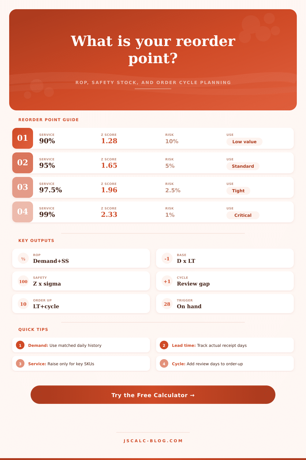
| 95% | 1.65 | 5 in 100 cycles | Standard retail, ecommerce, and warehouse planning |
| 97% | 1.88 | 3 in 100 cycles | Important SKUs where missed sales matter |
| 97.5% | 1.96 | 2.5 in 100 cycles | Controlled replenishment with moderate risk tolerance |
| 98% | 2.05 | 2 in 100 cycles | Service commitments with limited substitute products |
| 99% | 2.33 | 1 in 100 cycles | Critical parts, medical supplies, or high penalty misses |
🚚Supplier variability comparison grid
📋Supplier risk reference table
| Supplier profile | Multiplier | Use when | Planning note |
|---|---|---|---|
| Stable supplier | 0.70x | Receipts land close to promise dates | Lower lead-time sigma may be reasonable after clean history |
| Normal supplier | 1.00x | Most orders are on time with a few slips | Good default when measured lead time data is limited |
| Variable supplier | 1.35x | Lead times jump during busy or short-stock periods | Raise safety stock or split sourcing for high movers |
| Import or port risk | 1.75x | Customs, ocean freight, or port congestion affects receipts | Review order cycle and inbound pipeline together |
| New vendor | 1.50x | There are few completed purchase orders to measure | Start conservative, then reduce after repeatable receipts |
| Expedite lane | 0.55x | Premium freight or local pickup shortens uncertainty | Useful for temporary recovery, not a normal replenishment model |
🔁Order cycle quick table
| Order cycle | Cycle stock added | Common setting | Effect on order-up-to level |
|---|---|---|---|
| 0 days | 0 x daily demand | Continuous review or auto-replenishment | Order-up-to roughly equals ROP |
| 3 days | 3 x daily demand | Twice-weekly purchasing | Small top-up for the next review gap |
| 7 days | 7 x daily demand | Weekly purchase run | Common balance between workload and stock coverage |
| 14 days | 14 x daily demand | Biweekly vendor minimums | Order-up-to rises quickly for fast movers |
| 30 days | 30 x daily demand | Monthly imports or wholesale buys | Requires more cycle stock and stronger demand history |
🗂Preset comparison table
| Scenario | Daily demand | Lead time | Service level | Why it matters |
|---|---|---|---|---|
| Coffee beans | 42 units | 14 days | 95% | Daily movement with moderate supplier variability |
| Skincare jars | 18 units | 21 days | 97% | Batch production and packaging delays can stack up |
| Spare parts | 3.5 units | 35 days | 99% | Low demand but high downtime penalty |
| Clinic supplies | 64 units | 10 days | 99% | Higher service target for operational continuity |
| Bakery flour | 95 kg | 4 days | 95% | Fast replenishment but high daily usage |
| Apparel SKU | 7.8 units | 28 days | 90% | Seasonal demand can make overstock costly |
| Electronics kit | 12 units | 45 days | 98% | Long lead time and component availability risk |
| Warehouse case | 155 cases | 6 days | 95% | High-volume case movement needs clean rounding |
| Seasonal product | 26 units | 18 days | 97.5% | Demand volatility can overwhelm simple averages |
🧮Formula and method breakdown
| Step | Formula | What it means | Included inputs |
|---|---|---|---|
| Lead time demand | Average daily demand x lead time days | Expected usage while waiting for replenishment | Demand, lead time |
| Combined variability | Square root of lead and demand variance | Blends demand variability with supplier timing variability | Demand SD, lead SD, supplier profile |
| Safety stock | Z score x combined variability | Extra stock used to hit the chosen service level | Service level, variability |
| Reorder point | Average daily demand x lead time days + safety stock | Inventory position where a new order should be triggered | Demand, lead time, safety stock |
| Order-up-to level | Average daily demand x (lead time + cycle days) + safety stock | Target stock after accounting for the next review cycle | Order cycle, lead time, safety stock |
💡Inventory planning tips
Inventory management: The shelf appear to be stocked, right up until it’s not. That’s what keeps you up at night. You’ll look at the rack of spare parts or box of coffee beans and tell yourself there’s no reason to worry, plenty of time before you run low. Next thing you know, someone orders extra during a holiday sale, your supplier was late shipping by three days, and now you’re looking at a pile of backorders.
The reorder point is the line in the sand. It lets you know precisely when to place an order so that new batch just arrives when old one empties. The formula for this number isn’t guesswork. Calculating this threshold require accounting for average daily demand and time it takes for goods to travel from the dock to your shelf.
How to Calculate Your Reorder Point
However, the true challenge come with variation. When customer purchases is always consistent at 42 units and delivery times are always perfect at 14 days, you can input a fixed amount and go on your way. The world is not so clean. Lead times fluctuate because of port congestion or vendor backlogs. Marketing promotions and weather can cause demand fluctuations.
After plugging in your figures, the calculator above will do the math for you, eliminating boring algebra of squaring roots and standard deviations. Then it’ll boil down the madness into one actionable figure. And how much buffer you have are determined by which service level you select.
For most warehouses and retail operations, default setting is a service level of 95%. You’re fine with going out-of-stock about one time in every twenty times you need something restocked. Move that up to 99%, and your required safety stock go way up. And it doesn’t do so at a linear rate. It does so exponentially. This imposes a lot of pressure on your cash flow.
The tool let you instantly visualize this tradeoff. It allows you to see that when you ask for near perfect availability on something that has low margin, you are almost always paying more than the value of lost sale itself. Most people fail to realize this. They think everything you stock carries equal value. So if you go out-of-stock on a $200 gadget, that’s just an ego-bruising inconvenience. But if you run out of a $2 screw, you can kill a machine.
This is where supplier reliability comes into play so much. Do you have goods shipped across the ocean? You need to consider the inconsistency of freight and time it takes goods to pass through customs. You can adjust for supplier variability profiles by applying multipliers that reflect their actualy behavior. For example, if you have a reliable local supplier, then you might not need as many buffers compared to an unreliable overseas supplier.
Why does that matter? This prevents you from insuring too little against a risky lane (meaning you’re underinsured) or too much against a reliable one (you’re wasting capital by paying for insurance). The page has a reference table which outline these different behaviors of your suppliers and the impact on amount of stock you should hold.
It’s all about paying for certainty with your capital. It also changes the game when it comes to review cycles. Do daily inventory checks make you nimble? Or do you review monthly? In the latter case, your order-up-to level has to be way higher to fill the gap. That’s what they call cycle stock (versus safety stock).
Planners mix these up all the time. Safety stock is for the unexpected. Cycle stock is for the regular time between orders. Mix those up and you end up with an empty shelf or warehouse overflowing with slow moving stuff.
The quality of your data matters. GIGO means garbage in, garbage out. Did you have an unusually promotional period in history? Was there a shutdown? Your average will be skewed by that data. First, clean the history. What was the data like for the past six months to a year when things were running smoothly?
Measure lead time starting with confirmation of purchase order, not when it’s written. These are minor operational points but far more important than the formula itself. The input data matters. And since the math is only as good as the input, make sure that input is good.
So, all told, it’s about balance. How do you get the most availability of products for your customer but also minimize amount of cash sitting inside a box? There is no right answer. You can only find a defensible answer given the reality of your supply chain and your personal level of risk tolerance.
That’s what the calculator gives you. Clarity to do something vs. The paralysis to wait. If you don’t know where to begin, try some conservative assumptions, then update as you get actual receipts in. Eventually, the figures will firm up. What once felt like a mystery shelf will behave like a system. When you know the line you draw, the panic subsides.