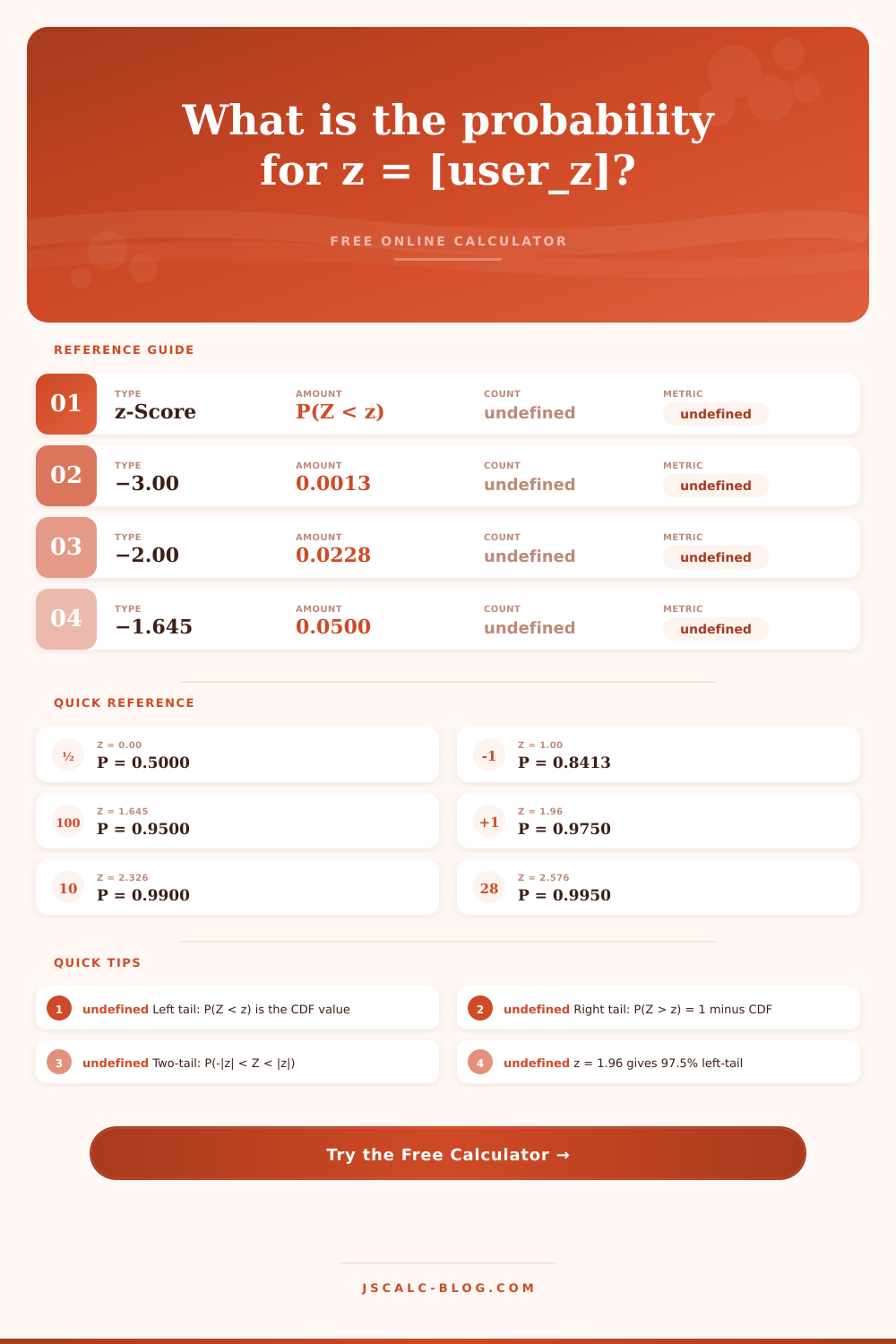
Probability Z Value Calculator
Enter a z-score and a probability mode to find the exact area under the standard normal curve. Supports left-tail P(Z < z), right-tail P(Z > z), and two-tail middle P(−|z| < Z < |z|). Uses the Hart rational approximation accurate to 7+ decimal places.
🎯 Common Z-Score Presets
📝 Inputs
Enter any value between −4 and 4. Negative z-scores are valid.
Left-tail is the standard CDF used in most z-tables.
📊 Quick Reference Z-Table
| z-Score | P(Z < z) Left-tail | P(Z > z) Right-tail | P(−|z|<Z<|z|) Two-tail | Common Use |
|---|---|---|---|---|
| −3.00 | 0.001350 | 0.998650 | — | 3-sigma lower tail |
| −2.576 | 0.005000 | 0.995000 | — | 99% CI lower bound |
| −2.326 | 0.010000 | 0.990000 | — | 98% CI lower bound |
| −1.960 | 0.025002 | 0.974998 | — | 95% CI lower bound |
| −1.645 | 0.050000 | 0.950000 | — | 90% CI lower bound |
| 0.000 | 0.500000 | 0.500000 | 0.000000 | Mean of distribution |
| 1.282 | 0.900000 | 0.100000 | 0.800000 | 80% two-tail CI |
| 1.645 | 0.950000 | 0.050000 | 0.900000 | 90% two-tail CI |
| 1.960 | 0.975002 | 0.024998 | 0.950004 | 95% two-tail CI (2-sided) |
| 2.326 | 0.990000 | 0.010000 | 0.980000 | 98% two-tail CI |
| 2.576 | 0.995000 | 0.005000 | 0.990000 | 99% two-tail CI |
| 3.000 | 0.998650 | 0.001350 | 0.997300 | 3-sigma rule |
🔢 Key Probability Landmarks
⚙ Hart Approximation Details
📋 Probability Modes Compared
| Mode | Formula | Typical z = 1.96 | Statistical Use |
|---|---|---|---|
| Left-tail P(Z < z) | CDF(z) | 0.975002 | Cumulative probability, percentile lookup |
| Right-tail P(Z > z) | 1 − CDF(z) | 0.024998 | Upper-tail p-values, one-sided hypothesis tests |
| Two-tail P(−|z|<Z<|z|) | 2 × CDF(|z|) − 1 | 0.950004 | Confidence intervals, two-sided hypothesis tests |
💡 Practical Tips
A z-score is a standardized measure of a data point. It represent how many standard deviations a particular value is away from mean. By doing so, we can begin to make comparisons between different kinds of data, if I got an 85 on my final exam and one on my easy quiz, these scores aren’t equal, right? But when converted to a z-score they are put on the same playing field; I can use the z-score to infer things about my score which is where statistics comes in. This website takes care of all that messy math required to convert that distance from the mean into something meaningful (you don’t have to fumble with integral or look up values in tables).
Here are a few things to note:
• The normal distribution is symmetrical, like a bell. This means that the probabilities will acts in expected ways. The calculator will show you the area under curve based off whatever z-score you enter. For most people, this begins with the left-tail probability. That’s the cumulative area from negative infinity to your point of interest.
• It corresponds to percentiles and can tell you what proportion of population sits below that value. If you’re above the mean by one standard deviation (i.e., a z-score of 1.0), then you’re above approximately 84% of the rest of the population.
What is a Z-Score and How to Use It?
But sometimes it’s worth considering the other side, aka the right tail when it comes to statistics. For example, hypothesis testing commonly use the chance that you’d see something as or more extreme than what you saw in the positive direction. This allows you to determine whether your result is statistically significant. When conducting a one-sided test for whether a new drug performs better then a placebo, you’re interested in the upper tail. This difference between the left and right tails are a subtle but important distinction that changes how we interpret significance and risk.
The other mode is the two-tail, which catches middle band between negative and positive z-values because that’s what forms the confidence intervals: A 95% confidence interval is not guessing, it’s a literal section of the center 95% of your results with 2.5% in each tail. This sort of understanding keeps you from accidently screwing up the alpha level (the chance you’re wrong). It prevents mistakes like confusing one-tailed versus two-tailed probabilities. Such mistakes would of result in your findings being wrong by half, which is bad in quality control or medical research.
You’ll notice that the tool visually shows you exactly which part of the bell curve are being sliced for you. This depends on some fancy math called the Hart (1968) rational approximation. It’s elegant and avoids having to rely on large numerical library code, while still giving you seven-decimal place accuracy. That’s important for things like 2.576 or 1.96, because very slight rounding can change the confidence level by significant amounts. You don’t have to remember the polynomial coefficients; just know that it’s a strong engine underneath which will help you believe what comes out of it.
The most common errors stem from confusion over which tail to apply to data; therefore, you must always first determine the question being asked. If it’s seeking a percentile rank, use the left tail. If it’s testing for superiority, examine the right tail. If it’s constructing an interval estimate, stay in middle with both tails. All three appear on the calculator at once so you can check your gut against the math and make the abstract world of statistics concrete.
At its heart, learning about z-scores (and other tools) is about taking a hard look at that thing we call “probability,” which are a way of expressing our own uncertainties, not an objective truth. The beauty of the tool is that it makes calculation easy, and then you interpret its results in light of your own situation. For example, you might be working with exam grades, manufacturing defects, or clinical trial data. Whatever it may be, the bell curve will always serve as a point of comparison. Seeing just how neatly it maps onto actual probabilities helps dissolve some of the angst around math because you can better understand what’s actualy happening here.