Probability Distribution Calculator
Pick binomial, Poisson, normal, or geometric, enter the parameters, and get P(X=k), P(X≤k), P(X≥k), the mean, and the variance with a full formula breakdown for each model.
🎲Real Distribution Presets
📝Distribution Inputs
Used by the binomial model only.
Upper bound when condition is between.
🔢Symbol Snapshot
📊Distribution Formulas & Moments
| Distribution | PMF or PDF | Mean | Variance | Support |
|---|---|---|---|---|
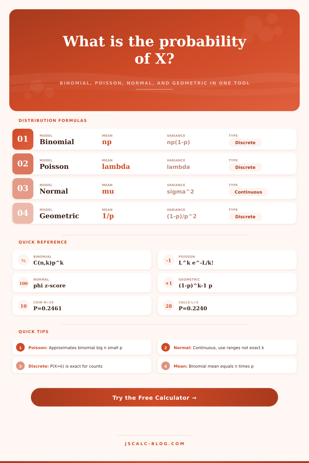
| Binomial(n, p) | C(n,k) p^k (1-p)^(n-k) | np | np(1-p) | k = 0, 1, …, n |
| Poisson(λ) | λ^k e^(-λ) / k! | λ | λ | k = 0, 1, 2, … |
| Normal(μ, σ) | (1/(σ√(2π))) e^(-(x-μ)²/(2σ²)) | μ | σ² | all real x |
| Geometric(p) | (1-p)^(k-1) p | 1/p | (1-p)/p² | k = 1, 2, 3, … |
🗂When To Use Each Distribution
| Distribution | Counts What | Key Assumption | Example | Shape |
|---|---|---|---|---|
| Binomial | Successes in n fixed trials | Fixed n, constant p, independent | Heads in 10 flips | Bell near np |
| Poisson | Events in a fixed interval | Constant average rate λ | Calls per hour | Right skewed |
| Normal | Continuous measurement | Symmetric around μ | Heights, IQ, errors | Symmetric bell |
| Geometric | Trials until first success | Independent trials, constant p | Rolls to first six | Decreasing |
⚖Binomial vs Poisson vs Normal
| Feature | Binomial | Poisson | Normal | Geometric | Data Type |
|---|---|---|---|---|---|
| Random type | Discrete | Discrete | Continuous | Discrete | — |
| Parameters | n, p | λ | μ, σ | p | — |
| Mean | np | λ | μ | 1/p | Center |
| Variance | np(1-p) | λ | σ² | (1-p)/p² | Spread |
| Range | 0 to n | 0 to ∞ | -∞ to ∞ | 1 to ∞ | Support |
| P(X=k) meaning | Exact successes | Exact count | Density only | First success | — |
| Approximates | Normal if np≥10 | Binomial big n | Limit of sums | Memoryless | — |
📋Common Parameter Presets
| Scenario | Distribution | Parameters | Mean | Variance |
|---|---|---|---|---|
| 10 coin flips | Binomial | n=10, p=0.5 | 5 | 2.5 |
| Calls per hour | Poisson | λ=3 | 3 | 3 |
| IQ scores | Normal | μ=100, σ=15 | 100 | 225 |
| First six on a die | Geometric | p=0.1667 | 6 | 30 |
| Sixes in 6 rolls | Binomial | n=6, p=0.1667 | 1 | 0.833 |
| Test scores | Normal | μ=75, σ=10 | 75 | 100 |
⚙Full Formula Breakdown
💡Practical Probability Tips
Imagine that you’re faced with a machine with 10 binary switches. You want to know the probability that if you flip every switch, you’ll get a specific pattern of heads and tails. “Intuitively, you’d think there’s a 50% chance of ending up with five heads. That isn’t right. This is where probability distributions come into play, they offer useful information for real-world decisions. In this case, the calculator crunches the numbers for you while leaving you to interpret the results.” “It calculates the combinatorics; you don’t have to do any fancy math.
This is a binomial situation… A fixed number of trials where there are two possible outcomes. For example, if you poll people, this would be useful for counting the number of yes answers. If you’re manufacturing products, it’s helpful for determining whether they meets a certain quality standard. While binomial has a fixed number of trials, Poisson counts events over time or space.
Simple Guide to Probability Distributions
The tool asks for the number of trials and the probability that each one is successful. Based off those inputs, the calculator finds the chances of achieving any given target level. It also returns mean (what you can expect on average) and the variance (how much you should expect to vary). When setting quality control limits, the variance is even more important than the mean.
Poisson: If you’re counting events in space or time instead of successes, then you switch to Poisson. Think of typos per page or calls per hour for customers. In this case, the key assumption is that the events occur independently with an average rate (constant). If there are many opportunities but each has a low chance of happening, then this is a good model.
In these instances, it’s also approximating the binomial distribution, so you don’t need to compute enormous combinations. Poisson distributions assumes mean = variance, making it easier to analyze if you have information about the average rate.
Continuous variables are things that can take on a range of values, such as your height, your weight, or a test score. Since you’re working with a continuous variable, by definition there’s a 0% chance of getting any specific number. Instead, we need to ask for ranges. How do we get those? Well, what does the calculator actualy do? It calculates the area under the curve from one point to another. And since many natural things tend to cluster around their average, this creates a bell shape.
Why do so many things cluster around an average? Welcome to the Central Limit Theorem.
A geometric distribution is a type of distribution. Geometric distribution is concerned with waiting time for the first success. Each trial must be independent, and there are no memories of past failures, it’s a memoryless process. An example would be rolling a die until you roll a six. As the number of failures increases, the probability of reaching the first success on a specific trial decreases. It is right-skewed.
It is useful when dealing with time-to-failure (reliability engineering) or anything else that involves time-to-first-success.
To know what distribution applies, you have to consider how your data’s structured. If it has a binary outcome and fixed number of trials then binomial probably applies. If you’re counting rare events over some interval then poisson will be right. For a continuous and symmetric variable, normal seems like the right choice. The page contains a reference table that makes this clear, presenting the models’ parameters and support.
The median and the mean are frequently confused. They’re equal when a distribution is symmetric (such as the normal). But for skewed distributions such as the geometric or Poisson, they differ. The mean, what the calculator gives you; is also called the “expected value.” That’s what you’d use to plan.
For example, if your call center typically gets three calls per hour, then that’s the number you’d use as your basic staffing level. But keep in mind the variance. Sometimes the mean looks good but the variance is high, causing wide swings that could swamp your staff. Because one input is so consequential: altering even a single variable can change the whole shape of probabilities.
In geometric models, for example, a tiny uptick in the chance of success cuts down a lot on the waiting time expectation. Even a tiny jump in the rate lambda widens the Poisson distribution, so far-out observations are less shocking. Understanding these sensitivities tells you what risks really matter.
What’s probability? Probability isn’t a crystal ball that predicts the future. It’s a way to measure our uncertainty and use it to make better decisions. If you manage risk, engineer something, or gamble, having some idea of what your odds look like puts you at an advantage. You’ll still throw those switches at random, but now you have a precise understanding of just how unlikely your lucky streak realy is.”