Price Elasticity of Demand Calculator
Estimate how quantity demanded responds when price changes. Choose midpoint or point elasticity, compare old and new revenue, classify demand, and see the formula steps behind the result.
🎯Demand Elasticity Presets
🧮Price and Quantity Inputs
Midpoint is best for two observed price and quantity points.
Context adjusts interpretation notes, not the elasticity formula.
Currency is for display only; elasticity is unit-free.
Use the same time period for both quantity entries.
Price before the observed change.
Units, seats, orders, or signups at original price.
Price after the change, discount, test, or promotion.
Matched quantity observed after the price change.
Applies only to the quantity change, useful for scenario checks.
Remove committed or contract quantity from both points if needed.
🔢Current Elasticity Snapshot
📐Formula Breakdown
📋Preset Comparison Grid
| Scenario | Original P/Q | New P/Q | Price Change | Qty Change | Approx Ed | Revenue Signal | Common Reading |
|---|---|---|---|---|---|---|---|
| Streaming plan increase | 12.99 / 48000 | 14.99 / 43500 | +14.3% | -9.8% | -0.69 | Revenue up | Inelastic in this band |
| Coffee shop menu test | 4.50 / 920 | 4.95 / 850 | +9.5% | -7.9% | -0.83 | Revenue up | Moderately inelastic |
| Airfare sale response | 320 / 1450 | 260 / 2140 | -20.7% | +38.4% | -1.85 | Revenue up | Elastic leisure demand |
| Commuter fuel shift | 3.60 / 118000 | 4.05 / 111500 | +11.8% | -5.7% | -0.49 | Revenue up | Short-run inelastic |
| E-book discount | 9.99 / 6800 | 6.99 / 12600 | -35.3% | +59.8% | -1.69 | Revenue up | Promotion-sensitive |
| Concert ticket drop | 85 / 6200 | 70 / 8500 | -19.4% | +31.3% | -1.61 | Revenue up | Elastic event demand |
| Utility basic use | 0.18 / 380000 | 0.21 / 365000 | +15.4% | -4.0% | -0.26 | Revenue up | Essential-use inertia |
| Luxury accessory markdown | 240 / 310 | 180 / 690 | -28.6% | +76.0% | -2.66 | Revenue up | Highly elastic |
| SaaS seat price test | 29 / 12200 | 34 / 10850 | +15.9% | -11.7% | -0.74 | Revenue up | Sticky but monitored |
🧭Elasticity Classification Reference
| Absolute Ed Range | Classification | Quantity Sensitivity | Revenue When Price Rises | Typical Examples |
|---|---|---|---|---|
| 0.00 | Perfectly inelastic | No measured response | Rises with price | Locked-in quantity, rare in practice |
| 0.01 to 0.49 | Very inelastic | Small quantity response | Usually rises | Short-run fuel, basic utilities |
| 0.50 to 0.99 | Inelastic | Less than price change | Often rises | Subscriptions, staples, commute needs |
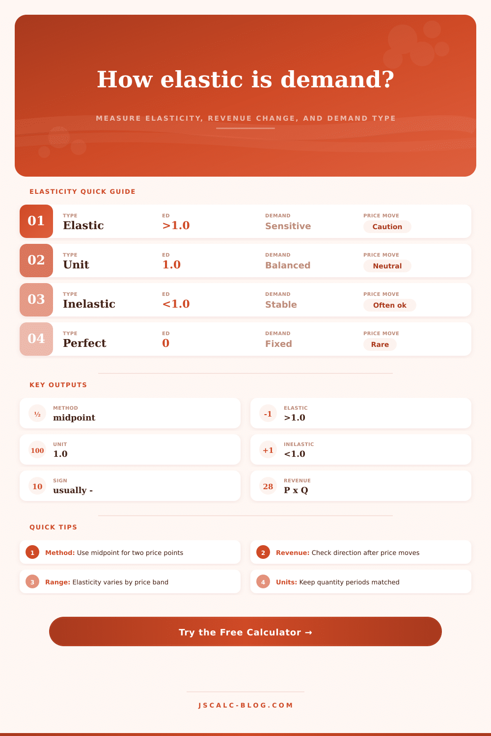
| About 1.00 | Unit elastic | Matches price change | Little change | Boundary cases, balanced tests |
| 1.01 to 1.99 | Elastic | More than price change | Usually falls | Travel, entertainment, digital promos |
| 2.00 and higher | Highly elastic | Strong response | Often falls sharply | Luxury goods, easy substitutes |
⚖Method Selection Guide
| Method | Formula Core | Best Use | Main Caution | Calculator Setting |
|---|---|---|---|---|
| Midpoint arc elasticity | % change using averages | Two observed price points | Blends the whole range | Midpoint arc |
| Point elasticity | Slope × P1 / Q1 | Local estimate around start point | Direction depends on base point | Point from start |
| Simple percent method | %Q / %P from old value | Fast rough explanation | Not symmetric | Shown in snapshot only |
| Regression elasticity | Log quantity on log price | Many observations over time | Needs controls and clean data | Outside this calculator |
| Cross elasticity | %Q item A / %P item B | Substitute or complement study | Different demand question | Use separate model |
| Income elasticity | %Q / % income | Demand versus income changes | Not a price response | Use separate model |
🔍Demand Data Quality Checks
| Check | Good Sign | Risk Sign | Why It Matters | What To Do |
|---|---|---|---|---|
| Matched period | Both quantities use same time window | One value weekly, one monthly | Elasticity is distorted by period mismatch | Normalize quantities first |
| Stable product mix | Same product or bundle compared | Bundle, size, or feature changed | Quantity response may not be from price | Separate product changes |
| Promotion overlap | No major campaign shift | Discount plus new ad push | Marketing can mimic price sensitivity | Tag or exclude promo effects |
| Inventory available | Supply could meet demand | Stockouts or sold-out days | Observed quantity caps true demand | Remove constrained periods |
| Competitor movement | Market prices were steady | Major rival price change | Substitution effects can dominate | Add market notes |
| Seasonality | Comparable demand season | Holiday or weather swing | Timing can bias elasticity | Compare like-for-like periods |
💡Practical Elasticity Tips
Go to your local coffee shop, watch as line gets longer, then notice latte goes up fifty cents in price. Magic? Nope. Economics. That’s what happens when the price elasticity of demand kicks in. This is the measure of how much consumers care about price compared to value of product.
While simple in theory, there’s a lot of complexity behind it. Business owner usually guess at it. They slash their costs and hope profits goes up, but they don’t. Or they raise prices and hope no one leaves, but it rarely make a difference. This page do the math for you, so you’ll stop guessing and start knowing.
How to Calculate Price Elasticity of Demand
So how do we know if our customers’ demand is inelastic (they will keep paying) or elastic (they’ll leave and find another option)? It depends: does raising prices generate a sufficient amount of margin to offset lost sales? If so, the demand is inelastic. Raising your prices won’t hurt business. People will still buy. Why? Because they don’t have any other choice, or because they really, truly need what you’re selling.
If not, the demand is elastic. Increasing prices will alienate too many customer to make up the difference in margin. Why? Because there’s a better alternative available, your customer cares enough about this purchase that they won’t accept your new price tag.
To do that, you only need two numbers, one at the start, another after a change. Tell the tool how much you paid and how many items you bought. Then tell it what those same numbers are today. Finally, hit the button.
By default, the tool will use midpoint method. This is key. Lots of people just take the number they want to measure (price, quantity) and divide it by its starting point. That’s asymmetrical. You’ll get one number if you think the change was a hike; another if you think it was a drop. Midpoint takes the average of both numbers, specifically the midpoint of prices and the midpoint of quantities. It makes calculation stable, providing a consistent benchmark across markets.
Take for example an increase in your monthly subscription cost from $12 to $15. That’s a modest increase, but it could cause a drop in subscribers. The demand would then be considered inelastic. Sales decrease by some percentage, yet revenues increases by more than the amount of reduction. Company wins!
Or consider offering a special discount on e-books. It could boost sales sky high, because demand is highly sensitive. You make up for the reduced price-per-unit with a huge increase in volume. Both strategies can be profitable; they just require different metrics to justify them. Using the calculator, you’ll know how much the demand has changed (the elasticity coefficient) as well as the revenue impact. Instant bottom-line effect: check.
The most obvious mistake is that people mix different time periods. For example, if your original data is in weekly sales and you switch to monthly sales for your new data, it will mess up the elasticity calculation. Normalizing the time period are crucial.
Another error is ignoring external factors. Did you raise your price while a competitor lowered theirs? Did you run a marketing campaign that made more people know your brand around this time? All these factor can blur results. Fortunately, you can adjust settings within the tool to smooth out noisy data. This helps you isolate the true price response instead of just seeing what happens in a busy market.
Elasticity isn’t fixed either. It varies with your location on the demand curve. At a very low price point, perhaps the customer sees the product as a great deal; so it’s inelastic. Increase the price sufficiently, though, and they start hunting around for alternatives and voila! It is now elastic. And that’s another reason it makes more sense to test small increments rather than make a huge leap all at once.
The calculator allows you to use midpoint or point elasticity. Use midpoint if you’re trying to measure how a minor change affects something from two different observed states. Use point if you’re interested in measuring the impact of a slight tweak from some known starting point. Pick whichever fits your data.
All this really comes down to margin vs. Volume. The more price sensitive your customer base (the more elasticity), the more they will skew the scale towards volume over efficiency. The more loyal and/or captive they are (less sensitive to price), the more they’ll weigh in direction of margin and value. The numbers don’t lie (they just need some context). Take a look at the outcome, see which way it moves revenue, and ask yourself if it’s right for your brand. Getting familiar with that demand shift is the first step towards smart pricing. It transforms a hunch into a strategy.