Population Growth Calculator
Project future population with exponential continuous, exponential annual, and logistic growth models. See doubling time, total growth, year-by-year curves, and the time it takes to reach a target size.
🌍Real Growth Presets
📝Growth Inputs
Use a negative value for a shrinking population.
Ignored when solving for time to a target.
Upper limit the environment can support.
🔢Formula Snapshot
📈Year-by-Year Projection
| Step | Time | Population | Growth This Step | Cumulative Growth | Multiple of Start |
|---|---|---|---|---|---|
| Enter values above to build the projection table. | |||||
🔬Growth Model Reference
| Model | Formula | Shape | Best For | Long-Run Limit |
|---|---|---|---|---|
| Continuous exponential | P = P0 × e^(r×t) | J-curve, smooth | Bacteria, compounding, short bursts | Grows without bound |
| Discrete exponential | P = P0 × (1 + r)^t | J-curve, stepwise | Annual census, yearly percent growth | Grows without bound |
| Logistic | P = K / (1 + A×e^(–r×t)) | S-curve, levels off | Cities, wildlife, limited resources | Approaches K |
| Linear (for contrast) | P = P0 + b×t | Straight line | Fixed additions each period | Grows without bound |
| Decline (negative r) | P = P0 × e^(–|r|×t) | Decay curve | Shrinking towns, die-off | Approaches zero |
⏳Doubling Time by Growth Rate
| Rate / Year | Continuous ln2/r | Discrete log2/log(1+r) | Rule of 70 | Multiple in 50 yr |
|---|---|---|---|---|
| 0.5% | 138.6 yr | 138.9 yr | 140.0 yr | 1.28× |
| 1% | 69.3 yr | 69.7 yr | 70.0 yr | 1.64× |
| 2% | 34.7 yr | 35.0 yr | 35.0 yr | 2.69× |
| 3% | 23.1 yr | 23.4 yr | 23.3 yr | 4.38× |
| 5% | 13.9 yr | 14.2 yr | 14.0 yr | 11.5× |
| 7% | 9.9 yr | 10.2 yr | 10.0 yr | 29.5× |
| 10% | 6.9 yr | 7.3 yr | 7.0 yr | 117× |
🌎Growth Rate Examples
| Scenario | Start | Rate | Model | Horizon | Notes |
|---|---|---|---|---|---|
| Growing city | 100,000 | 2.0% | Continuous | 50 yr | Steady urban expansion |
| Bacteria culture | 1,000 | 25% | Continuous | 24 hr | Rapid, hour-scale doubling |
| Country census | 8,000,000 | 0.9% | Discrete | 30 yr | Annual census reports |
| Wildlife with cap | 500 | 12% | Logistic | 40 yr | K limits the herd size |
| Shrinking town | 25,000 | –1.0% | Continuous | 50 yr | Out-migration decline |
| Startup users | 5,000 | 8% | Discrete | 10 yr | Monthly cohort growth |
| World population | 8,100,000,000 | 0.9% | Logistic | 80 yr | Slowing toward a ceiling |
⚙Full Formula Breakdown
📋Reference Values
| Symbol | Meaning | Typical Entry | Where It Applies |
|---|---|---|---|
| P0 | Starting population | 10 to 8 billion | All models |
| r | Growth rate as a decimal | –0.02 to 0.30 | All models |
| t | Elapsed time in units | 1 to 200 | Future population mode |
| K | Carrying capacity ceiling | Above P0 | Logistic only |
| N | Target population | Above P0 to grow | Time-to-reach mode |
💡Practical Growth Tips
Exponential growth mean you begin with a tiny amount of bacteria or people. Then you apply a moderate rate of increase. What happens? It explodes out of control in just a few decade. It’s slow to start, then all-consuming. That’s why most predictions is flawed, we don’t make the transition from linear thought to exponential fact. I’ve built a calculator that do the math for you. But it’s less important than knowing when to apply which type of model.
The first trap that folks fall into is thinking about whether to use a discrete model (change occurs in steps, e.g., once per year) vs. A continuous model (change occur continually, e.g., interest compounds continuously). In many situations, this doesn’t matter: if you’re looking at something far off into the future, a continuous model will be close enough to its discrete counterpart. If you’re trying to account for short bursts, though, then the model could mislead your expectation. It supports both; jump from stepwise changes to smooth curves and back again while keeping an eye on which trend you’re following. When working with numbers as different than urban planning metrics and biological expansion, that flexibility make all the difference.
How Growth Models Work
Eventually, however, things gets crowded. Resources is limited. Competition arise. Nothing expands unchecked. That’s when the logistic model kicks in. It still starts off with an exponential curve, but adds a carrying capacity, a concrete cap on the potential population level. As it nears that cap, the curve flattens, bends and slows. A real system can’t support unlimited fish in a lake or cities sprawling across the ocean. In reality, most do not (though they might come close). Selecting the logistic option require setting this limit, anchoring the projection to the physical world instead of theoretical.
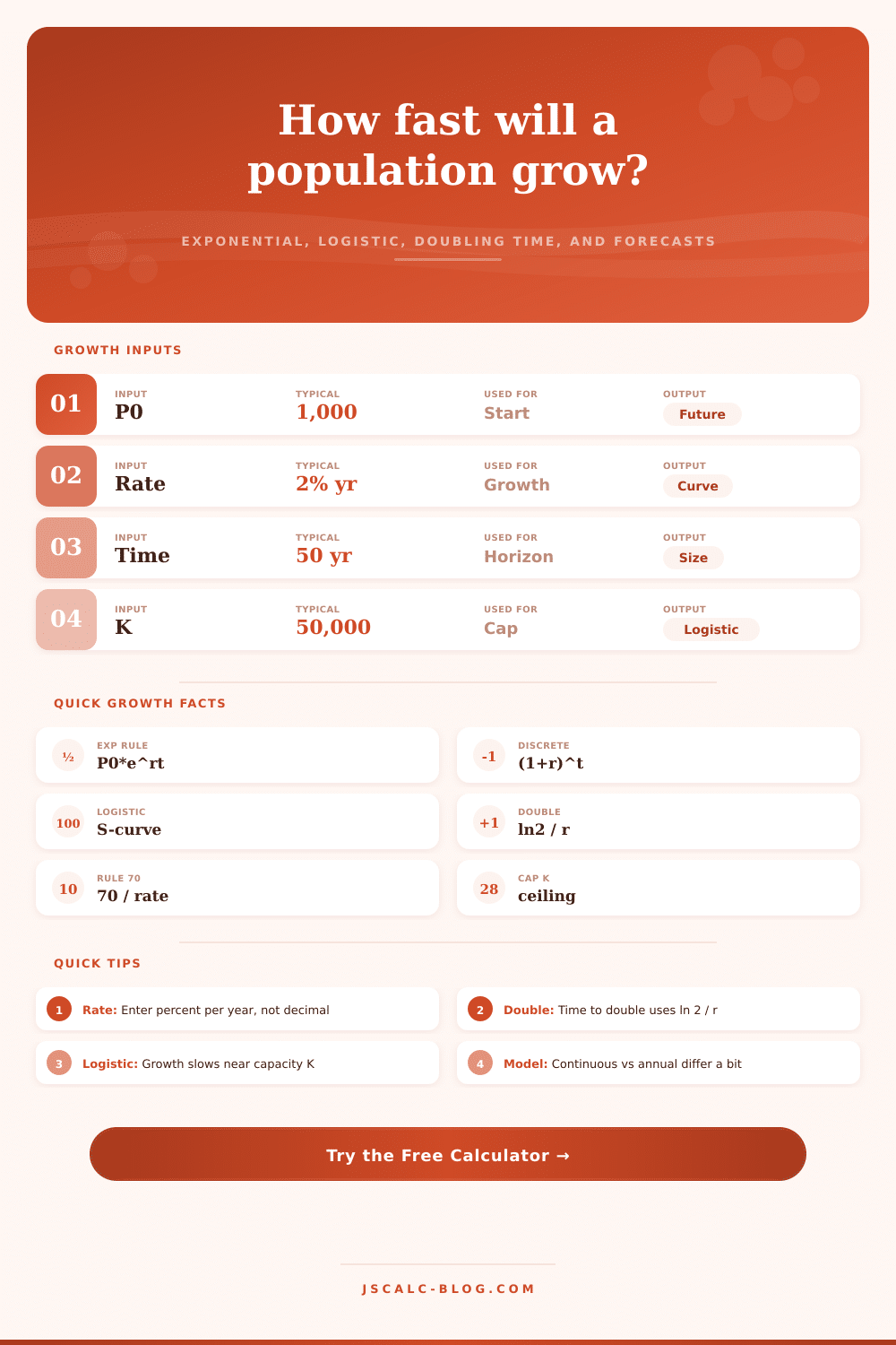
Please share this. Any rate you input gets a fast sanity check: what’s the double time? One percent annually? Your population will double every seventy years. Two percent? It halves that to thirty-five. Five percent? That shortens it to fourteen years. Those are abstract numbers until you think of all the infrastructure that needs to be built. If a town doubled in size, it would of need double the water supply, double the number of schools, and double the number of hospitals. This isn’t a linear problem; it’s exponential. It is exponentially harder then linear. With mismatched capacity and timing, it break. The table on the page spells it out and shows just how big a difference a few percentage points can make on the timeline.
Long-term trends matter more than short-term changes: We tend to underestimate their effects while overestimating those of the latter. Sure, one bad harvest won’t reverse half-a-century’s worth of gains. But who knows? Maybe a small drop in the birth rate will seem negligible now, yet cause major shrinkage across four generations’ time. Shrinking cities follows negative-growth decay curves, which work every bit as effectively as positive ones. And yes, calculator shows you both types equally well.
Output is only as good as input: Typing in a rate of 0.02 instead of two percent would be an easy error to make. The calculator assume you want the percentage number itself to avoid the headache of converting from a decimal. If your rate period is annual, it needs annual time units. Similarly, if you use months, then your inputs should also be measured in months. Otherwise you’ll add noise that distracts from signal. Spend a few seconds checking that the units you’ve selected for time are consistent with your rate period before clicking the calculate button.
All in all, it’s not really an arithmetic problem, it’s a trajectory problem. Population growth isn’t what happens; it’s where we’re headed. The numbers tell you where you are heading; the model tells you why. The curve will explain everything, from global population trends to the rise of startup users and even the size of a herd of wild animals. Exponential lines promise endless expansion. Logistic curves hum warnings of limited resources. Knowing which one matter shifts your thinking about tomorrow.
Start with a small figure, add a gentle rate and see: the outcome explodes beyond control in just a couple of decades. That’s the odd magic of exponential growth.