Pearson Correlation Significance Calculator + Critical r

Pearson Correlation Significance Calculator

Decide whether a correlation r is statistically significant by comparing it to the critical r value for your sample, then read a Fisher r-to-z confidence interval for the true correlation.

📌Real Correlation Presets

📝Correlation Inputs

Correlation coefficient r (–1 to 1)

The observed Pearson r from your two variables.

Sample size n (pairs)

Number of paired observations. df = n – 2.

Significance level α (for critical r)

Test tail

Confidence level for the CI

Decimal places

Enter r and n to test significance.

Significant? — compares |r| with critical r

Critical r 0 threshold for this n and α

t-statistic 0 with df degrees of freedom

Confidence interval for ρ 0 Fisher r-to-z interval

🔢Key Quantities

n – 2Degrees of freedom

r²Shared variance

n – 3Fisher SE base

|r|Compared to r_crit

📊Critical r by Sample Size

Sample n	df (n – 2)	Critical r at α=0.05	Critical r at α=0.01
5	3	0.878	0.959
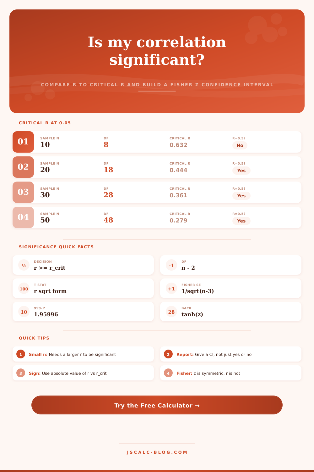
10	8	0.632	0.765
15	13	0.514	0.641
20	18	0.444	0.561
25	23	0.396	0.505
30	28	0.361	0.463
40	38	0.312	0.403
60	58	0.254	0.330
100	98	0.197	0.256
120	118	0.180	0.234

🗂Sample Size vs Decision Grid

Sample n	df	r_crit 0.05	r_crit 0.01	r=0.5 at 0.05	r=0.5 at 0.01
8	6	0.707	0.834	Not sig	Not sig
12	10	0.576	0.708	Not sig	Not sig
16	14	0.497	0.623	Sig	Not sig
20	18	0.444	0.561	Sig	Not sig
30	28	0.361	0.463	Sig	Sig
50	48	0.279	0.361	Sig	Sig
80	78	0.220	0.286	Sig	Sig
100	98	0.197	0.256	Sig	Sig

🔄Fisher r-to-z Transform

r value	z = atanh(r)	r value	z = atanh(r)
0.10	0.100	0.60	0.693
0.20	0.203	0.70	0.867
0.30	0.310	0.80	1.099
0.40	0.424	0.90	1.472
0.50	0.549	0.95	1.832

📏Effect Size & Decision Rules

\|r\| Range	Effect Size	r² Shared	Rule
0.00 to 0.10	Negligible	0% to 1%	Sig only with very large n
0.10 to 0.30	Small	1% to 9%	Needs large n to reach r_crit
0.30 to 0.50	Moderate	9% to 25%	Often sig near n = 20 to 40
0.50 to 0.70	Large	25% to 49%	Usually sig by n = 15 to 20
0.70 to 1.00	Very large	49% to 100%	Sig even with small n

⚙Full Formula Breakdown

Degrees of freedomdf = n – 2. A sample of n = 20 pairs gives df = 18 for the t distribution.

t-statistict = r × sqrt((n – 2) / (1 – r²)). For r = 0.5 and n = 20 this is about 2.449.

Critical tt_crit is the t value for df at the chosen α and tail, read from a built-in table with interpolation.

Critical rr_crit = t_crit / sqrt(df + t_crit²). For df = 18 at α = 0.05 two-tailed, r_crit ≈ 0.444.

DecisionThe result is significant when |r| ≥ r_crit. r = 0.5 clears 0.444, so it is significant.

Fisher transformz = 0.5 × ln((1 + r) / (1 – r)) = atanh(r). This stretches r onto a near-normal scale.

Standard errorSE = 1 / sqrt(n – 3). For n = 20 the SE of z is about 0.2425.

Interval in zz ± z_crit × SE, where z_crit = 1.95996 for a 95% interval, 1.64485 for 90%, 2.57583 for 99%.

Back-transformr_low and r_high = tanh(z ± z_crit × SE). This returns the interval to the r scale.

📋Reference Values

Item	Symbol	How It Is Used	Typical Value
Two-tail z 95%	z_crit	Half-width of Fisher CI	1.95996
Two-tail z 90%	z_crit	Narrower Fisher CI	1.64485
Two-tail z 99%	z_crit	Wider Fisher CI	2.57583
Fisher SE	SE	Spread of z estimate	1 / sqrt(n – 3)
Critical t (df 18)	t_crit	Feeds r_crit at 0.05	2.101

💡Interpretation Tips

Small samples need bigger r: With n = 10 the critical r at α = 0.05 is about 0.632, so even a moderate r near 0.5 fails the test. Larger samples lower the r threshold quickly.

Report a CI, not just a verdict: A significant result only rules out zero. The Fisher r-to-z interval shows the plausible range for the true correlation, which is far more informative than a bare yes or no.

People fail to recognize that if they gets a correlation coefficient of 0.5, there must be a strong relationship between those two variable. Not so fast! Correlation is just a number, which requires comparing against the sample size from which it originated. Often, knowing how many data points you have will tell you difference between signal and noise. This tells you if you can claim statistical significance to say the pattern are real instead of random. To know for sure, you must test for significance.

There’s just one problem: What constitutes “moderate” depends a lot on your sample size. In a huge dataset, an otherwise-unnoticeable correlation will be washed out; in a small study, something that barely squeaks by can look like a moderate effect. Once you enter your sample size into the calculator (above), it’ll do the math for you, no need to wrestle with inverse hyperbolic functions and flip through t-distribution tables yourself. It’ll test your actual r against some sort of critical threshold (which varies based off your degrees of freedom). If your absolute r value passes this threshold, then the relationship is statistically significant. You’ve got a pass/fail gate there.

Why Sample Size Matters for Correlation

But again, real wisdom comes in nailing the inputs. How strict should we make it? Well, the answer is “it depends” on sample size. If you have only ten pairs, then you’ll need an r around 0.63 (at traditional levels of confidence) to even barely clear the bar. It is a high bar indeed. Small samples is naturaly unstable, and a single data point out of place can throw its r-value all over the place. The further you grow your sample, however, the quicker that bar falls. For example, an r of 0.28 is sufficient for significance when you get up to fifty observations. And here’s the thing: this explains why larger scale studies shows statistically-significant correlations so often that they appear almost trivial.

Even if the true relationship among the variables are too weak to care about in the real world, a tiny r with a massive n will still clear the bar. But a significance test can only inform you that the correlation is not zero. It doesn’t say anything about how strong it is or if it’s important at all. So much better to report the confidence interval: Is it positive? Yes. How strong? Not sure. We have an interval in which true population correlation probably lies. And the Fisher z-transform helps make those intervals more accurate by straightening the skewed distribution of correlation coefficients so they look like a normal one.

Inverse tangents and logarithms scare most people away from this step, but the confidence interval range it creates tell you a lot more than just yes or no. It provides a margin of error for how strong your relationship is. It is not a binary flag. Be careful too about the distinction between practical importance vs. This is statistical significance. It’s possible for a study to show that studying correlates with test scores by 0.15 and with a sample size of ten thousand that’ll certainly be statistically significant. But it likely won’t enable you to predict how someone will do.

Look to shared variance (r squared) as a way to get some perspective. An r of 0.3 explains only nine percent of the variation in outcomes. Everything else accounts for the other ninety-one percent. If you don’t look at effect size, you’re overvaluing your weak findings by chasing significance.

Two other factors move the probability around: One- vs. Two-Tailed Testing. In some cases (e.g., if you have a good theory that predicts a positive effect), a one-tailed test is stronger since it puts all of your uncertainty on one side. But by default, most people use two-tailed tests out of caution. That’s safer but requires higher scores. Before running the calculator, be sure to choose the correct tail; the calculator will then set the critical value accordingly.

No matter how low your p-value is, it is still correlation rather than causation. It could be that the number of people who drown rises perfectly with the sale of ice cream, but that doesn’t mean one causes the other; it simply means that they both increases during the summer. Calculation never beats context. Run the numbers to confirm your pattern, but use your judgement to understand what it says. The numbers can tell you whether there is something going on here; you should of determined whether or not it’s worthy of listening to.