P-Value From T-Score Calculator
Convert a Student t statistic and degrees of freedom into left-tailed, right-tailed, or two-tailed p-values, then compare the result with alpha and the matching critical t cutoff.
📌Presets
Enter a t statistic and degrees of freedom to calculate the p-value.
⚙T Distribution Inputs
Use the t statistic from your test and the matching degrees of freedom. Two-tailed p-values use p = 2 x (1 - CDF(abs(t))).
📋Live Tail Breakdown Grid
🧭Current Test Snapshot
📚Reference Tables
| Tail choice | p-value formula | Critical comparison | Reject H0 when | Typical wording |
|---|---|---|---|---|
| Left-tailed | CDF(t) | t <= tcrit(alpha) | p <= alpha | Statistic is unusually low |
| Right-tailed | 1 - CDF(t) | t >= tcrit(1 - alpha) | p <= alpha | Statistic is unusually high |
| Two-tailed | 2 x (1 - CDF(abs(t))) | abs(t) >= tcrit(1 - alpha/2) | p <= alpha | Statistic is unusually far from zero |
| Near zero | tail area near 0.5 or 1 | inside critical bounds | usually not rejected | Observed t is ordinary under H0 |
| Wrong sign one-tail | large p near 1 | opposite side of cutoff | usually not rejected | Effect points the other way |
| Extreme t | small tail probability | beyond selected cutoff | often rejected | Rare under the null model |
| Degrees of freedom | t 90% two-tail | t 95% two-tail | t 99% two-tail | t 95% one-tail | t 99% one-tail |
|---|---|---|---|---|---|
| -- | -- | -- | -- | -- | -- |
| Example | t statistic | df | Tail | p-value | Alpha decision |
|---|---|---|---|---|---|
| Mean difference | 2.10 | 24 | Two-tailed | 0.0464 | Reject at 0.05 |
| Left-tail audit | -1.85 | 15 | Left-tailed | 0.0421 | Reject at 0.05 |
| Right-tail trial | 2.50 | 30 | Right-tailed | 0.0091 | Reject at 0.01 |
| Small sample | 1.40 | 6 | Two-tailed | 0.2110 | Do not reject |
| Large df | 1.97 | 180 | Two-tailed | 0.0504 | Just above 0.05 |
| Wrong sign | -2.00 | 20 | Right-tailed | 0.9704 | Do not reject |
| Input source | How df is often found | t statistic source | Tail selection cue | Calculator action |
|---|---|---|---|---|
| One sample t-test | n - 1 | (mean - mu0) / SE | mean differs, greater, or less | Enter reported t and df |
| Paired t-test | pairs - 1 | mean difference / SE | average change direction | Use paired-test df |
| Two sample pooled t | n1 + n2 - 2 | mean gap / pooled SE | group gap direction | Use pooled-test df |
| Welch t-test | Welch-Satterthwaite | mean gap / Welch SE | group gap direction | Fractional df is allowed |
| Regression coefficient | residual df | estimate / standard error | coefficient sign | Use model-reported df |
| Correlation test | n - 2 | r converted to t | association direction | Use correlation-test df |
🧮Formula Notes
The value of t-statistic represents a distance, but it’s a distance in units called “standard errors.” It is also point on a curve whose shape depends upon your sample size. It doesn’t tell you if something are significant by its value alone. For that, you need p-value.
The p-value takes this abstract distance and turns it into a judgment of whether it is signal or noise. Noise? The number of degrees of freedom also influence the shape of the distribution. Specifically, it relate to the heaviness of tails.
Understanding P-Values and T-Tests
For example, with smaller samples, the t-distribution have fatter tails different than a normal curve. Therefore, there’s more chance that you’ll observe extreme values from random chance. So you must consider this. But if you ignore your degrees of freedom, you’re assuming that your sample was infinitely large, and that’s not often true.
The nice thing about using the calculator is that it do all this for you. You don’t need to consult those printed-out table!
Which tail? Consider carefuly. If you don’t expect any difference in either direction, use a two-sided test. It’s safe.
If you suspect a specific direction, increase your ability to find it by using a one tailed test (which carries more risk). However, if you get results that aren’t what you expected, you might dismiss them as nothing at all even though they are a huge effect in the other direction. Many people falls into this trap. They select their tail AFTER looking at result. That makes the whole thing invalid.
It shows you all three options. Left, right and two tails; side by side. You can watch the p-value shift under each of these assumptions.
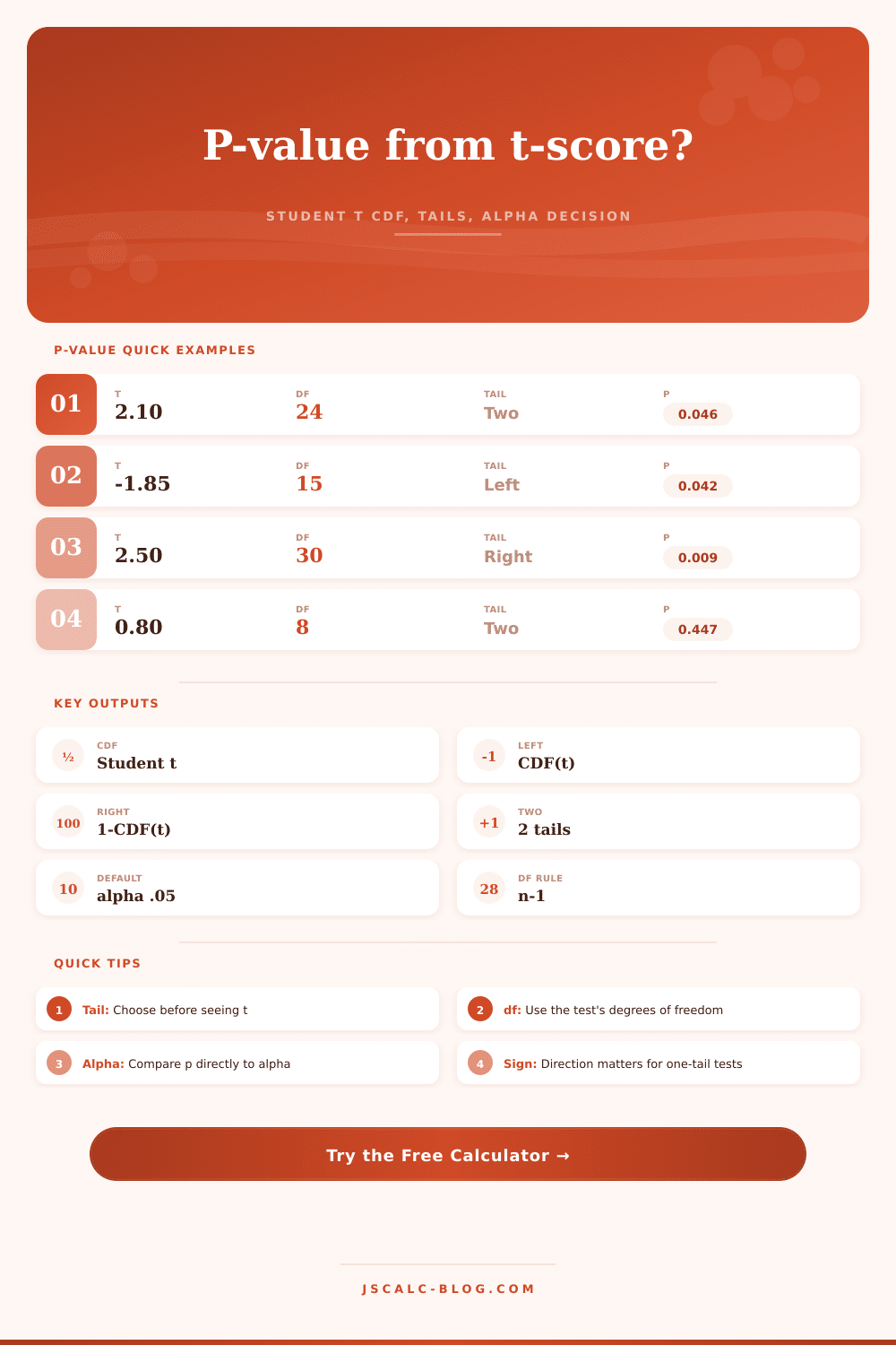
Now let’s say we have a t-statistic of 2.10 with 24 degrees of freedom. That translates into about a p-value of 0.046 in a two-tailed test. It is significant at the.05 level, but it is barely significant.
What if we alter the degrees of freedom to 6? Not as impressive. The key cutoff shift outwards. You can see that in the reference table. It shows just how the margin of rejection alters based off sample size.
The p value isn’t absolute either. It is relative to the number, the sample size, and an alpha level. A lot of folks think of p-values as on-off buttons: off is “not significant” and on is “significant.” Instead, they should of been thought of as gradations of evidence.
P = 0.05 is different than P = 0.049 only because we’ve arbitrarily defined it that way. There’s no naturaly data-driven distinction between them. You get exactly how likely something is. Then you decide for yourself how strong the evidence are. That matters if you’re trying to make decisions in areas such as policy or medicine. A false positive might cost a lot, know how far you are from the cliff.
Uncertainty matter with small sample sizes, which the t-test handles. A t-test never prove that your hypothesis is correct. Rather, it measures the amount of surprise you’d feel if your null hypothesis was actualy true. Once you understand this, you’ll see the p-value as a measure of surprise. That helps calm your nerves.
You won’t fret so much over the 0.05 cutoff. Instead, you’ll focus on size and direction of the effect. The mathematics sets the boundary. You decide what it means. The statistics becomes a story.