P-Value From Chi-Square Calculator

Calculate chi-square p-values for direct statistics, goodness-of-fit counts, or contingency tables with right-tail, left-tail, and explicitly defined two-tail reporting from JSCalc-Blog.com.

🧪Descriptive Presets

⚙Chi-Square Inputs

Input source

Reported tail

Chi-square statistic, x

Use the test statistic already computed from your study, model, or variance test.

Degrees of freedom, df

For standard tests this is positive; non-integer df are allowed for some approximations.

Observed category counts

Enter comma-separated counts, such as 72, 28 or 118, 96, 84, 102.

Expected counts or probabilities

Use counts, percentages, or probabilities. Values summing near 1 or 100 are scaled to the observed total.

Estimated parameters subtracted from df

Use 0 for fixed expected proportions; use 1+ when parameters were fitted from the same data.

Contingency table counts

Rows separated by semicolons; columns separated by commas. Example: 34,46,20; 50,40,10.

2 x 2 continuity correction

Table orientation note

Significance level, alpha

Displayed precision

Reported p-value

0.000000

right-tail

Chi-square statistic

0.0000

Degrees of freedom

distribution parameter

Decision at alpha

Check

based on selected tail

📌Current Distribution Snapshot

0.050

Right-tail Q

0.950

Left-tail P

7.815

Right critical x

3.000

Distribution mean

🔢Formula Breakdown

Distribution: if X follows a chi-square distribution with df degrees of freedom, then X is Gamma(shape = df/2, scale = 2).

Right-tail p-value: p = Q(df/2, x/2), where Q is the regularized upper incomplete gamma function.

Left-tail probability: p = P(df/2, x/2), where P is the regularized lower incomplete gamma function and P + Q = 1.

Two-tail option here: p = min(1, 2 x min(P, Q)). Chi-square tests usually use the right tail, so use this only when you intentionally want a doubled extremeness check.

Goodness-of-fit statistic: x = sum((observed - expected)^2 / expected), with df = categories - 1 - fitted parameters.

Contingency table statistic: expected cell = row total x column total / grand total, x = sum((observed - expected)^2 / expected), df = (rows - 1)(columns - 1).

📘Right-Tail Chi-Square Critical Values

df	alpha 0.10	alpha 0.05	alpha 0.01	alpha 0.001
1	2.706	3.841	6.635	10.828
2	4.605	5.991	9.210	13.816
3	6.251	7.815	11.345	16.266
5	9.236	11.070	15.086	20.515
10	15.987	18.307	23.209	29.588
20	28.412	31.410	37.566	45.315
30	40.256	43.773	50.892	59.703

🧭Which Tail Should Be Reported?

Reported tail	Formula used	Common use case	Decision direction
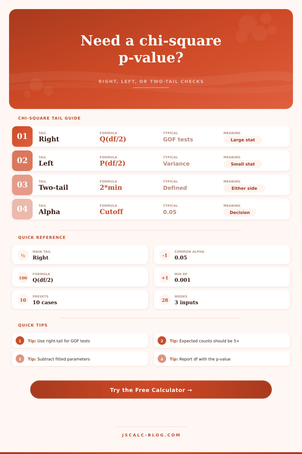
Right-tail	Q(df/2, x/2)	Goodness-of-fit, independence, homogeneity, residual deviance	Large x is more surprising
Left-tail	P(df/2, x/2)	Lower variance checks, unusually small dispersion, minimum variability questions	Small x is more surprising
Two-tail defined	2 x min(P, Q), capped at 1	Deliberate extremeness checks when both small and large statistics matter	Either tail can be flagged
Critical-value view	Compare x to inverse CDF	Auditing a p-value against a textbook table	Reject when p is at or below alpha
Effect-size view	Use x with sample size where relevant	Contingency tables and category fits	Separates practical size from significance
Simulation check	Empirical tail frequency	Very sparse expected counts or custom sampling designs	Use when asymptotic assumptions are weak

📋Chi-Square Test Use Cases

Test situation	Typical input	df rule	Main p-value	Important check
Goodness-of-fit	Observed and expected category counts	k - 1 - fitted parameters	Right-tail	Expected counts usually 5 or higher
Independence table	Rows by columns count table	(r - 1)(c - 1)	Right-tail	Rows and columns should be independent observations
Homogeneity table	Groups by outcome counts	(r - 1)(c - 1)	Right-tail	Same outcome categories across all groups
Variance test	(n - 1)s² / sigma²	n - 1	Tail depends on hypothesis	Data should be plausibly normal
Poisson dispersion	Residual deviance or Pearson statistic	model residual df	Right-tail	Compare against model assumptions
Log-linear model	Likelihood-ratio chi-square	model contrast df	Right-tail	Confirm nested model relationship

📊P-Value Evidence Comparison Grid

p-value band	Evidence label	At alpha 0.10	At alpha 0.05	At alpha 0.01	Reporting action
p > 0.10	Weak evidence	Do not reject	Do not reject	Do not reject	Report exact p-value and context
0.05 < p <= 0.10	Marginal	Reject	Do not reject	Do not reject	State the alpha threshold clearly
0.01 < p <= 0.05	Moderate	Reject	Reject	Do not reject	Include statistic and df
0.001 < p <= 0.01	Strong	Reject	Reject	Reject	Check expected counts before concluding
p <= 0.001	Very strong	Reject	Reject	Reject	Report as p < 0.001 if rounded
p near alpha	Borderline	Depends	Depends	Depends	Avoid rounding across the cutoff
p rounded to 0	Underflow risk	Reject	Reject	Reject	Use scientific notation

✅Actionable Checks

Before reporting: For category-count tests, inspect expected counts. A common rule is that every expected count should be at least 5, or sparse cells should be combined before relying on the chi-square approximation.

Before comparing: Match the tail to the hypothesis. Goodness-of-fit and independence tests are normally right-tail because larger chi-square statistics mean the observed pattern is farther from expectation.

A chi-square test calculates how far apart two sets of numbers are from each other. I.e., “observed” versus “expected.” This distance is translated into a statistic called a p-value. If the probability (i.e., the p-value) of observing that distance is low, then your observed pattern probably isn’t a fluke: you can reject the null hypothesis.

It also does all that complicated gamma function math for you with the calculator (above). Feed it your raw counts or statistics, and it spits out the probability. But remember: The tool will only be as good as the question you give it.

How to Use Chi-Square Test

Commonly, folks end up picking incorrect tail. Because these distributions is skewed to the right, they have a long tail of big numbers. That’s what most tests worry about (large deviations). If the observed data are really far away from the expected data, then its statistic will also be realy big. So the right tail is the usual one. It says, What is the probability I’d get a number like this or bigger? And if that number is less then your alpha (typically 0.05), you say you rejected the null.

The other lever are degrees of freedom (which aren’t just made up on the fly). It’s how many different thing can be varied independently. For example, for a contingency table, you subtract one from the number of rows and columns then multiply those results. For a goodness-of-fit test, it’s the number of categories minus one, minus however many parameters you estimate from your own data. The latter part is key: if you estimated the expected proportions from your data, you don’t get as much room to test how well they fit. Failing to adjust for this make your significance level bigger, so it will look like you found something when all you’ve got is noise.

As you can see from the reference table on the page, critical values move around based off degrees of freedom. That’s why, with low degrees of freedom, even a small chi-square statistic will become significant. Because the distribution spreads out and flattens as the degrees of freedom increase, it takes much more of a statistic to indicate significance, there are simply more possibilities for your data to deviate in a way that happens purely by chance. This is why you get so many statistically significant finding from enormous datasets that have no practical meaning. Findings like a connection between sunburns and ice cream sales might seem significant, but they aren’t because sunburns do not actualy cause people to eat more ice cream. They just happened in enough places that it seems unlikely to be random.

But don’t take it at face value; always double-check your expected values. Each cell need to behave normally for the chi-square approximations to work. When any of your expected counts fall beneath five, math falls apart. Your p-values are probably inaccurate, and so too are the probabilities. It’s better to combine some categories here or try another test (Fisher’s exact). The calculator spits out a number either way, but it’s up to you to decide if that number make sense.

There’s a nuance in interpreting what it outputs. There isn’t such a thing as “true” (a p-value of 0.04) or “false” (one of 0.06). It’s a spectrum of evidence. Something just above the line may well require a little more data to reach significance, something just over may be tenuous. The arbitrary cut-off is less important than context. When testing a new drug, you’d like rock-solid evidence. When looking at whether your manufacturing process has drifted a bit, you may be OK with a more relaxed standard. You get the probability. Your job is to judge.

But that’s ultimately what statistics are: learning to live with uncertainty. And if the chi-square test shows a pattern in your categorical data, that’s great. That’s one way to sift through the noise and find the signal. But remember its assumptions, use the correct number of degrees of freedom, make sure each cell contains sufficient data, and (for most tests) use the right tail. Then the p-value will be meaningful and not just guesswork. Then the chi-square test would of revealed to you the shape of truth underneath the numbers.