P-Value From F Statistic Calculator
Find upper-tail, left-tail, or two-tail-style F-test probabilities for ANOVA, regression, nested-model, and variance-ratio work on JSCalc-Blog.com.
Use the reported F value. F must be zero or greater.
Examples: MS between, added-model SS/df, or larger sample variance.
Examples: MS within, residual MSE, or comparison sample variance.
Overall F = (R² / p) / ((1 - R²) / (n - p - 1)).
ANOVA groups minus 1, predictors, added parameters, or sample 1 df.
Usually residual, within-group, error, or sample 2 df.
Use 1 for standard equal-variance or equal-mean-effect tests.
| Quantity | Formula | Typical source | Use in decision |
|---|---|---|---|
| Direct F statistic | reported F | ANOVA or regression output | Compare to critical F and p-value |
| Mean square ratio | MS numerator / MS error | ANOVA table | Upper-tail p-value |
| Variance ratio | s1² / s2² | Two sample variance test | Often two-tail style if direction was not planned |
| Regression overall F | (R²/p) / ((1 - R²) / (n - p - 1)) | Model summary | Tests whether predictors improve fit |
| Upper-tail p-value | 1 - CDF(F) | ANOVA, regression, nested models | Reject when p < alpha |
| Two-tail style value | 2 x min(CDF, 1 - CDF) | Variance-ratio checks | Use when both high and low ratios matter |
| Context | Observed ratio | df1 meaning | df2 meaning | Tail style | Common alpha |
|---|---|---|---|---|---|
| One-way ANOVA | MS between / MS within | groups - 1 | N - groups | Upper | 0.05 |
| Two-way ANOVA term | MS term / MS error | term df | error df | Upper | 0.05 |
| Overall regression | MS regression / MSE | predictors | n - p - 1 | Upper | 0.05 |
| Nested regression | added SS per df / MSE full | added predictors | full model error df | Upper | 0.05 |
| Variance ratio | s1² / s2² | n1 - 1 | n2 - 1 | Two-tail style | 0.05 |
| ANCOVA term | MS adjusted term / MS error | term df | adjusted error df | Upper | 0.05 |
| Screening design | factor MS / residual MS | factor df | residual df | Upper | 0.10 |
| Repeated contrast | contrast MS / error MS | contrast df | error df | Upper | 0.05 |
| Design | Numerator df1 | Denominator df2 | Example |
|---|---|---|---|
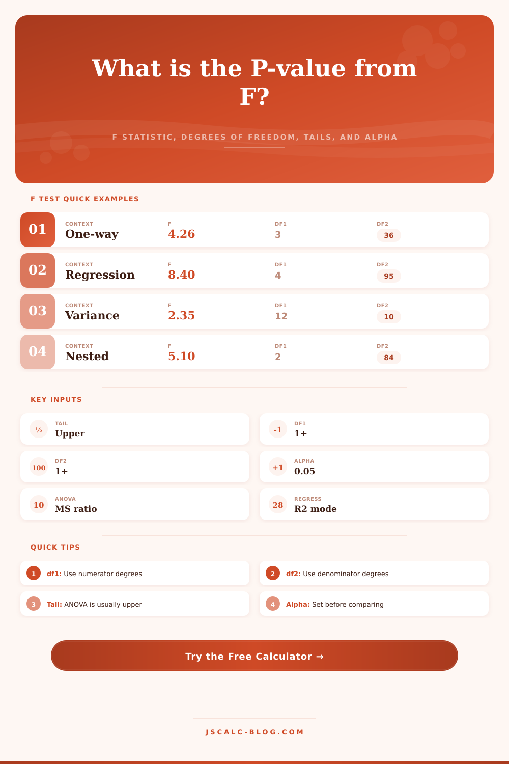
| One-way ANOVA with k groups | k - 1 | N - k | 4 groups, 40 total: df1 = 3, df2 = 36 |
| Overall regression | p predictors | n - p - 1 | 4 predictors, n = 100: df1 = 4, df2 = 95 |
| Added predictors test | p full - p reduced | n - p full - 1 | 2 added, full error df 84: df1 = 2, df2 = 84 |
| Two sample variance ratio | n1 - 1 | n2 - 1 | 13 and 11 observations: df1 = 12, df2 = 10 |
| Single ANOVA factor term | levels - 1 | model error df | 3-level factor with error df 54: df1 = 2, df2 = 54 |
| Interaction term | (a - 1)(b - 1) | error df | 3 x 2 design: df1 = 2 times 1 = 2 |
| P-value range | Evidence against null | Decision at alpha 0.05 | Plain reading |
|---|---|---|---|
| p < 0.001 | Very strong | Reject null | Observed F is far into the selected tail |
| 0.001 to 0.01 | Strong | Reject null | Result is uncommon under the null model |
| 0.01 to 0.05 | Moderate | Reject null | Meets the common 5 percent threshold |
| 0.05 to 0.10 | Weak to suggestive | Do not reject at 0.05 | May matter in planned screening work |
| p ≥ 0.10 | Limited | Do not reject | Observed ratio is not unusual enough |
| Two-tail style | Depends on both tails | Compare selected p to alpha | Useful when unusually small or large ratios count |
So now you’ve got it, the F statistic. You see this number in your spreadsheet and it’s bold. But what does it mean? That’s when most of us stop our analysis. Does this number seem big enough? Did I do something right with my experiment?
The calculator above perform the math for you, converting the raw ratio to a probability you can trust. To understand why that probability matters though, you must move beyond just seeing the number. An F statistic is basicly a signal-to-noise ratio. It’s a test of how much the group difference (or whatever else your model explains) account for the variation as compared than random leftover noise. As the signal grow stronger, the ratio rises. When the noise prevails it remains close to one. Understanding what that number measures are the key.
What the F Statistic Means and How to Use It
This is not a test of truth. It tests whether pattern you see would be unlikely to happen by chance alone, if there were no pattern to begin with. That’s what keeps you from claiming more than your data warrants.
The real work come in getting the degrees of freedom right. Those are the numbers that determine shape of the distribution curve behind the math. You can think about the numerator as the degrees of freedom of your model: how complex is it? And then you have the denominator, which take into account both your sample size and that degree of model complexity. Get those mixed up, and you get a different number out. A little detail, yes; but it matters.
If you run a regression on a hundred observations with four predictors, that denominator get you ninety-five degrees of freedom. There’s some wiggle room there to make the test slightly more sensitive. Run the same regression with just two groups from a tiny lab study, and now the denominator is smaller. Now the bar for significance are higher. The tool will adjust accordingly, it’ll handle all this automatically. But it needs you to feed it the right counts.
The tail is also context-dependent. Upper tails is typically used for most ANOVA tests (you’re looking for big ratios). You care whether group means are way apart. That’s not how variance tests work. Either variance might be bigger; you have less reason to assume one direction, so the two-tail approach make more sense. The calculator has a setting for this. Set it beforehand. Changing your mind after you’ve seen the outcome is called “data snooping,” and statisticians frown upon it. Be rigid rather than clever at this stage.
That’s your pre-commitment: the alpha level. It’s arbitrary, 0.05 is standard, but that’s just a choice. You have to decide and do so prior to running the test or you’ll chase significance forever. Want to require stronger evidence? Set your alpha lower. How about 0.01?
The p value indicates how far away from zero your observed F are along the probability curve. Is it rare if the null were true (low)? Or is it common (high)? It doesn’t prove the null is true; it only fails to reject it. Headlines miss that important nuance.
But think practicaly. What if you’re doing a quality control test and want to know how much variation there is between two machine-produced part? Or you’re testing three ad campaigns that convert at different rates in marketing. Same math. Different interpretation. Always, are you looking at structure or randomness? That’s what the F test is all about.
This page has a handy reference table of sorts that will help you align your test type with the right parameters. Beware of cherry picking: The F test is sensitive to normality. The p value becomes fishy if there’s a lot of skew in your data. There are no calculators for fixing poor data. They are only for processing what you feed them. So clean up your data first. Verify your assumptions. Then use the tool.
It helps you avoid having to lookup values on a table yourself. It minimizes transcription errors. Automation = accuracy.
In the end, then, the F statistic is the bridge. It’s what joins your raw numbers to an answer. And the price of passage is the p value. Feed in the proper ingredients and you recieve an accurate reply. You should of used better data if you want results. If you don’t care about which tail, or about degrees of freedom, then you’re not really using the tool; you’re only guessing.
The calculator takes away the friction. It allows us to concentrate on the story the data offers, not how we combined it. From a ratio, you begin. To a judgment, you arrive. In-between is where stats resides.