Null Hypothesis Rejection Calculator
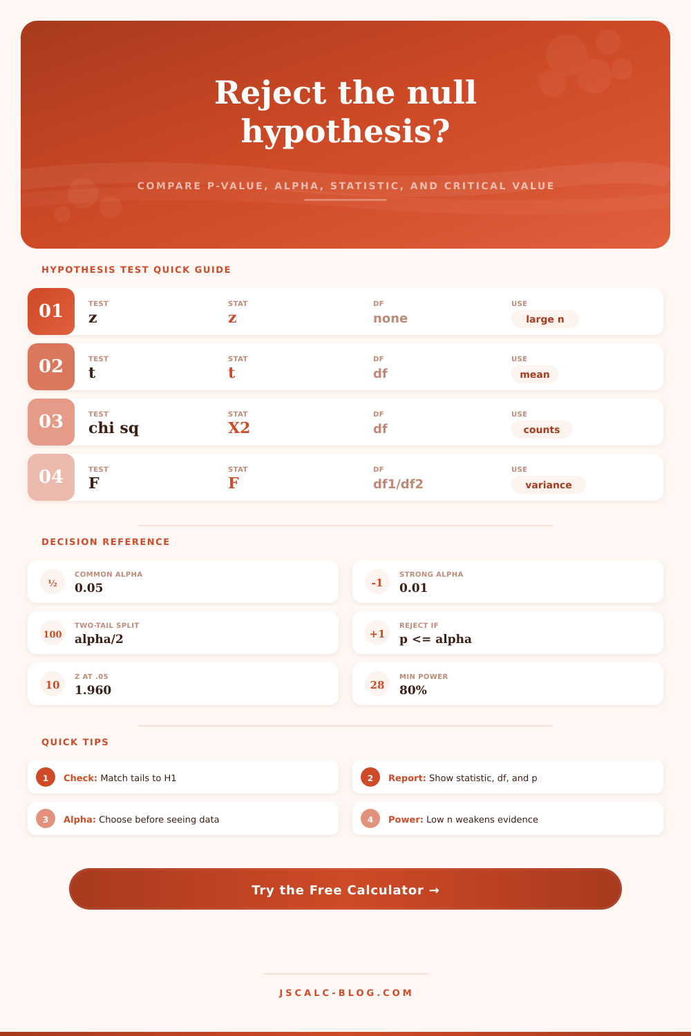
Compare p-value against alpha and test statistic against the critical region for z, t, chi-square, and F tests. Choose the distribution, tails, degrees of freedom, effect direction, sample size, and statistic source to decide whether to reject H0.
🎯Hypothesis Testing Presets
📝Test Inputs
Use z for known standard error or large-sample proportions, t for estimated standard error, chi-square for counts, and F for variance or model tests.
Critical regions follow H1, not the visual direction of the observed effect alone.
Common choices are 0.10, 0.05, 0.01, and 0.001.
Effect-based statistic uses (estimate - null) / standard error for z or t tests.
Examples: z = 1.96, t = -2.10, X2 = 11.07, F = 4.35.
Leave blank to calculate p from the selected distribution and tails.
For t and chi-square this is df. For F this is numerator df.
Used only for F tests as denominator df.
Use this to sanity-check whether the tail choice matches the research claim.
Used for interpretation and approximate power notes.
Mean difference, conversion difference, coefficient, or other estimate.
Usually 0 for differences and coefficients, or the claimed benchmark value.
Needed only when the statistic is computed from the effect estimate.
This changes the wording of the interpretation and report line.
🔢Current Test Snapshot
📊Distribution Reference Table
| Test family | Typical statistic | Degrees of freedom | Null model | Critical rule |
|---|---|---|---|---|
| z test | z = estimate / SE | None | Standard normal when SE is known or n is large | Compare z to normal quantile |
| Student t test | t = estimate / SE | Usually n - 1 or model residual df | t distribution with heavier tails | Compare t to t quantile using df |
| Chi-square goodness-of-fit | X2 = sum (O - E)^2 / E | Categories - 1 - fitted parameters | Observed counts follow expected proportions | Usually right-tail X2 critical |
| Chi-square independence | X2 from contingency table | (rows - 1)(columns - 1) | Row and column variables are independent | Usually right-tail X2 critical |
| F variance ratio | F = s1^2 / s2^2 | df1 and df2 | Population variances are equal | Right-tail or two-tail F critical |
| F regression model | F = MS model / MS error | predictor df and residual df | All tested coefficients are zero | Usually right-tail F critical |
📐Common Alpha and Critical Values
| Alpha | Confidence | Two-tail z critical | Right-tail z critical | Decision wording |
|---|---|---|---|---|
| 0.10 | 90% | ±1.645 | 1.282 | Weak evidence threshold |
| 0.05 | 95% | ±1.960 | 1.645 | Most common research cutoff |
| 0.025 | 97.5% | ±2.241 | 1.960 | Stricter one-sided reporting |
| 0.01 | 99% | ±2.576 | 2.326 | Strong evidence threshold |
| 0.001 | 99.9% | ±3.291 | 3.090 | Very strong evidence threshold |
🧪Hypothesis Test Comparison Grid
| Scenario | Distribution | Tail | Statistic | DF input | Reject when |
|---|---|---|---|---|---|
| One-proportion A/B lift | z | Right or two | z score | None | p <= alpha or z beyond critical |
| Known-SE process mean | z | Left, right, or two | z score | None | Statistic falls in normal rejection region |
| Small sample mean | t | Left, right, or two | t score | n - 1 | t exceeds df-based critical value |
| Regression coefficient | t | Usually two | t score | Residual df | Coefficient differs from zero |
| Goodness-of-fit counts | Chi-square | Right | X2 | categories - 1 | X2 exceeds upper critical value |
| Independence table | Chi-square | Right | X2 | (r - 1)(c - 1) | Association is unusually large |
| Variance comparison | F | Right or two | Variance ratio | df1 and df2 | F outside critical bounds |
| Overall regression model | F | Right | MSR / MSE | model and error df | Model explains signal beyond noise |
🔍p-Value Evidence Reference
| p-value range | Evidence against H0 | At alpha 0.05 | Reporting phrase | Caution |
|---|---|---|---|---|
| p > 0.10 | Weak | Fail to reject | Not statistically significant | Could be low power |
| 0.05 < p <= 0.10 | Suggestive | Fail to reject | Marginal by 0.10 only | Avoid overclaiming |
| 0.01 < p <= 0.05 | Moderate | Reject H0 | Statistically significant | Check effect size |
| 0.001 < p <= 0.01 | Strong | Reject H0 | Strong evidence | Assess assumptions |
| p <= 0.001 | Very strong | Reject H0 | Very strong evidence | Still not proof |
⚙Formula Breakdown
💡Actionable Testing Tips
Statistical significance isn’t a light switch. Just because your p-value dips below 0.05 doesn’t mean your result is true, nor does it mean that your work are worthless if it stays above 0.05. That’s a binary way of looking at it but it misses the point of hypothesis testing.
Your test do not demonstrate that your theory is right. Rather, it informs you if the data you gathered is sufficiently surprising to cast some doubt on how things is. And if you do this, you should of consider the evidence, rather then chase a magical number alone.
Understanding Statistical Significance
The choice of distribution is where it begin. If you believe your sample is large enough (or you’ve measured its error), then use a z-test. If you don’t quite know what you’re doing, go ahead and admit it, just use a t-test and let the variation within your sample do the work. For categories and counts, turn to chi-square. For comparing variances, reach for an F-test.
Why? Because if the mechanics appears similar, the math underneath will fall apart. T-tests for means is used most often simply because they forgive most sins: you likely didn’t know the actual population variance. But tell it which door to walk through and calculator above will do the math for you.
The number you set for alpha is the threshold beyond which you’ll look at the data. It’s the cost of a false positive. If you set it to.05, then you’re saying you’ll cry wolf five percent of the time, even if it’s only the wind. Tighten that to.01 and you’ll need stronger proof. You will get fewer false alarms but you are also more likely to miss a true effect. It’s a tradeoff; you can’t have perfect sensitivity and perfect specificity at the same time. The page has a reference table laying all of this out, showing how different criteria tightens or loosen your critical values.
Decide what kind of error hurts more. Missing a cure is disastrous, while wasting time on a minor change to a button color are more costly in an A/B test.
People say a lot about tails. They don’t realize how important they is. With a one tailed test, you’re looking in one direction; with a two tailed test, you just care if there’s any difference at all. Once you peek under the curtain and learn which way the outcome went, switching to one or the other is simply cheating the system. If you think new process might be faster, you test to see if it’s faster. If you only care whether it’s different, then you test to see if it’s different. The p-value and the critical region both comes into play here to ensure that you remain honest.
Your calculator compares your statistic to the boundary where we would reject the null hypothesis, and if your statistic falls past this point, the null hypothesis are booted.
The price for parameter estimation is degrees of freedom. Whenever you compute a standard deviation or a mean from your data, you lose one degree of freedom. Fewer degrees of freedom means less sharpness, more width, and more flatness of the distribution. It requires a larger effect to get to significance, and it guards against concluding things based off noise. More degrees of freedom mean results are sharper and tighter with less width.
You can find statistical significance in very tiny differences, but being statistically significant does not means it matters in practice. Look at the effect size! You may discover a difference that is realy small (and no one cares). A decline of 0.1 percent of customer satisfaction might be technically true (statistically significant), but it’s completely useless.
The shadow side of significance is power. Your sample size is too small. You’ll still fail to reject the null, though the alternative is true. This is called a false negative. You didn’t make a claim, so it’s OK, but you may have. But how do you know you didn’t miss something? It will show you why your silence doesn’t mean nothing. It’s not telling you anything if you have a high p-value and low power. All it says is you didn’t look hard enough.
Uncertainty is managed with hypothesis testing; not eliminated. You collect the data, set the rules, and interpret results based on those rules. The numbers tell you what to do, but judgment seals the deal. Should you accept or reject? No. Understand. And then act, not just on/off, but how brightly does the light shine?