One Proportion Z-Test Calculator
Test one observed sample proportion against a claimed null proportion with tail-aware p-values, confidence intervals, assumption checks, and formula steps from JSCalc-Blog.com.
| Check | Rule of Thumb | Why It Matters | Calculator Field |
|---|---|---|---|
| Independent observations | Sampling method or randomization supports independence | Z formulas assume each trial does not set the next trial result | Study design outside the numeric inputs |
| Expected successes | n p0 is at least 10 | Normal approximation needs enough expected events under the null | Sample size and null proportion |
| Expected non-successes | n(1 - p0) is at least 10 | Both sides of the binomial need enough mass for z-test use | Sample size and null proportion |
| Outcome is binary | Each observation is success or non-success | The method is for one sample proportion, not a mean or count rate | Outcome label and context |
| Sample fraction | If sampling without replacement, n is no more than 10% of population | Large sampling fractions can reduce the true standard error | Study design note |
| Alternative | Question It Answers | P-Value Formula | Typical Use |
|---|---|---|---|
| Two-sided: p ≠ p0 | Is the proportion different from the benchmark? | 2 x P(Z ≥ abs(z)) | Audits, neutrality checks, unknown direction changes |
| Greater: p > p0 | Is the proportion higher than the benchmark? | P(Z ≥ z) | Conversion lift, completion gain, support majority |
| Less: p < p0 | Is the proportion lower than the benchmark? | P(Z ≤ z) | Defect reduction, churn reduction, incident drop |
| Confidence interval | What range of true proportions fits the sample? | p-hat +/- z* SE-hat | Reporting uncertainty and practical effect size |
| Use Case | Alpha or Confidence | Two-Sided Critical z | One-Sided Critical z |
|---|---|---|---|
| Loose screening | alpha 10% or 90% CI | 1.645 | 1.282 |
| Common report | alpha 5% or 95% CI | 1.960 | 1.645 |
| Stricter report | alpha 1% or 99% CI | 2.576 | 2.326 |
| Very strict report | alpha 0.1% or 99.9% CI | 3.291 | 3.090 |
| Scenario | Success Definition | Common Null p0 | Usual Tail | Watch First | Decision Note |
|---|---|---|---|---|---|
| Landing page experiment | Visitor signs up | Historical conversion | Greater | Independent visits | Use CI gap to judge practical lift |
| Factory defect audit | Unit is defective | Maximum allowed defect rate | Less | Clear defect rule | Low p-value supports defect reduction |
| Public opinion poll | Respondent supports option | 50% or previous poll | Two-sided or greater | Sampling frame | CI is often easier to explain |
| Delivery compliance | Order arrives on time | Service target | Less or two-sided | Definition of on time | Below-target tails should be planned |
| Email campaign | Email is opened | Baseline open rate | Greater | Duplicate recipients | Large samples can make small gaps significant |
| Training completion | Learner completes module | Goal completion rate | Two-sided or greater | Course access window | Compare p-value with completion target |
| Subscription churn | Customer churns | Target churn rate | Less | Same churn window | Report lower rates as absolute pp change |
| App reliability | Session has crash | Allowed crash rate | Less | Session independence | Rare-event settings may need exact methods |
| Null p0 | Minimum n for n p0 ≥ 10 | Minimum n for n(1 - p0) ≥ 10 | Practical Reading |
|---|---|---|---|
| 1% | 1000 | 11 | Rare events need large samples for z approximation |
| 2% | 500 | 11 | Useful for low defect or incident rates |
| 5% | 200 | 11 | Common for conversion and failure testing |
| 10% | 100 | 12 | Balanced enough for routine tests |
| 50% | 20 | 20 | Most efficient point for normal approximation |
| 95% | 11 | 200 | High pass rates need enough expected non-passes |
There’s a new landing page design you launch and see that it boosts conversion rate from five percent to seven percent. Huzzah! Your team cheers because the lift look good, and they’re eager to deploy it on the rest of site.
But that increase could simply be noise. The observed proportion is based off a tiny amount of data, which is randomly varying so as to look like an actual change. There’s no way to know if it’s true improvement. It could just be luck that a random string of visitor happened to sign up.
How to Use a One Proportion Z-Test
This is what the one proportion z-test helps with: does my sample proportion differ meaningful from some known benchmark? Here’s where math comes into play. It’s based on normal approximation to the binomial distribution. If your sample are big enough, the distribution of sample proportions will be centered around true population proportion with some knowable spread.
Plugging in your counts and target rate into calculator above lets it do all that math for you. No need for you to look up tail areas in a table or calculate standard errors by hand. All you have to do is enter three numbers: the total sample size, number of successes and the proportion that the null hypothesis says should exist. Then, it spits out z-score, which measures how many standard deviations your observed rate are from the expected baseline.
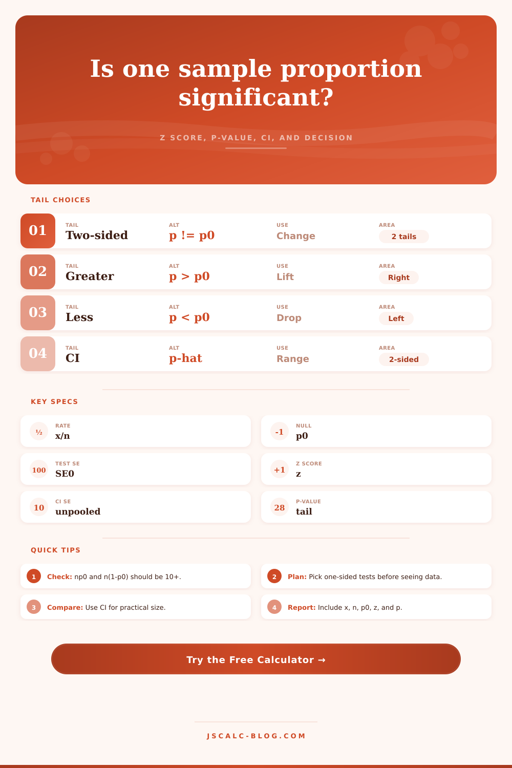
Most folks don’t appreciate that choosing which tail to use for your hypothesis matter. In a less-than test, you might hope the defect rate is down and audit for defects. A greater-than test would be used if you think new design works better. If you have no prior expectation as to direction of change then a two-sided test makes sense. Picking the tail based on what you see in data invalidates the p-value because now you’ve effectively cherry picked your hypothesis to fit results. The page lays it all out nicely in reference tables, note how the critical values will vary by alternative you select.
Rare events also tend to cause trouble for analyst who rely on sample sizes. Under the null hypothesis, the number of expected successes and expected failures must each be greater than 10 for the normal approximation to apply. For example, if your test involve a one-percent defect rate, then you will require a minimum of a thousand samples even to meet that preliminary condition. Otherwise, the distribution is skewed and the z-test become invalid; instead, you’ll have to use exact methods or collect more data. The calculator runs through these conditions for you and alerts you when there’s not enough data to draw valid conclusion.
Significance does not imply practical importance. Even with a large sample, smallest possible change could be highly statistically significant (e.g., a p-value smaller than.001) because it’s such a small fraction of a percent differenter. You could end up rejecting the null hypothesis at the cost of implementing something whose return doesn’t cover its cost.
That’s why it’s important to report both the p-value and confidence interval. The second provides a range of potential values for true proportion, so that you can evaluate size of the effect. If the interval is tight and it’s nowhere near the threshold, you have a strong result.
There is one slight difference in how the confidence interval and the test statistic are calculated for standard error. For the confidence interval, we use the observed proportion to calculate variation. This shows range of values given your observed data. But with the z-test, we estimate variation using the null proportion (what would of been expected if the null was true). That way we don’t double count the evidence when constructing both a point estimate and an interval, which would make our intervals too narrow. Most people won’t have to think much about this technical detail; the tool will automatically apply right formula to each result.
And lastly, think about what else is going on with your data. One caveat: You have to have independent observations. If one observation affects another (for example, due to a social network effect), then standard error formulas break down. Another caveat: You may need to use the finite population correction if you’re sampling a small number of items from a larger population. The calculator makes assumptions about normal random sampling conditions.
Ultimately we want to use a test to improve our decision and not just get a tiny p-value. If we get a statistically significant result then we know that change was probably real. The size of it? While the confidence interval gives us an idea of magnitude of the change, we should use it alongside the p-value to get a fuller picture. We don’t really need the p-value for this. We have the confidence interval, which gives us an idea of the size of the change. This combination gives a better picture then both metrics separately.
Instead of trusting your gut feeling about one data point, now you’re launching with conviction because the evidence backs it up. That’s what proper testing of proportions will do.