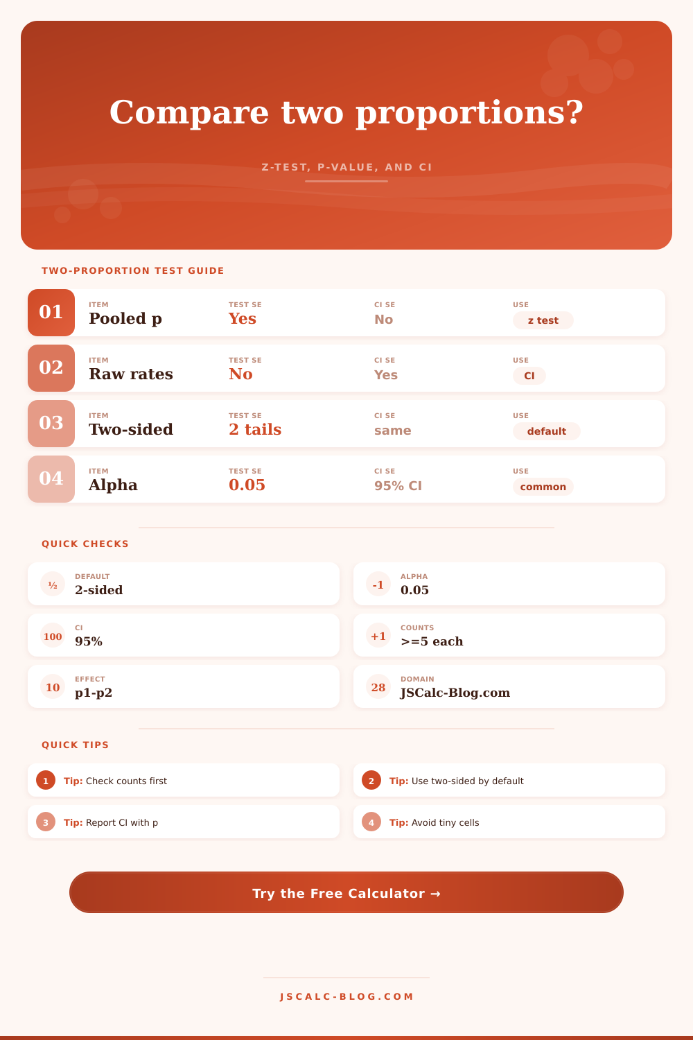
Two Proportion Z-Test Calculator
Compare two independent success rates with a pooled z-test, tail-specific p-value, and unpooled confidence interval from JSCalc-Blog.com.
Two-Proportion Results
| Use case | Group 1 | Group 2 | Success metric | Common tail | Watch before testing |
|---|---|---|---|---|---|
| A/B conversion test | New page | Current page | Signup, click, or purchase rate | Two-sided or greater | Random assignment and no duplicate visitors |
| Survey support | Current survey wave | Previous survey wave | Percent choosing a response | Two-sided | Comparable sampling frame and wording |
| Clinical response | Treatment group | Control group | Response or remission proportion | Two-sided | Independent participants and defined endpoint |
| Quality defect rate | New process | Old process | Defect, return, or failure rate | Less | Same inspection rules for both groups |
| Education intervention | Intervention class | Comparison class | Pass, mastery, or attendance rate | Greater or two-sided | Student independence and stable criteria |
| Product adoption | Exposed users | Unexposed users | Activated or retained users | Greater | Cohort timing and exposure definition |
| Risk monitoring | Site or period A | Site or period B | Incident or complaint proportion | Two-sided or less | Equal reporting threshold and complete records |
| Marketing creative | Creative A | Creative B | Click-through or lead rate | Two-sided | Allocation balance and campaign overlap |
| Alternative | Written hypothesis | P-value formula | Best used when |
|---|---|---|---|
| Two-sided | p1 - p2 != H0 difference | 2 × (1 - Phi(|z|)) | Any meaningful difference in either direction matters. |
| Greater | p1 - p2 > H0 difference | 1 - Phi(z) | You planned in advance to test whether group 1 is higher. |
| Less | p1 - p2 < H0 difference | Phi(z) | You planned in advance to test whether group 1 is lower. |
| Confidence level | Two-sided z* | Approximate central area | Typical pairing |
|---|---|---|---|
| 80% | 1.282 | Middle 80% | Exploratory screening with wider tolerance for misses. |
| 90% | 1.645 | Middle 90% | Directional product or operations reviews. |
| 95% | 1.960 | Middle 95% | Common reporting level for two-proportion comparisons. |
| 98% | 2.326 | Middle 98% | Higher caution when false positives are costly. |
| 99% | 2.576 | Middle 99% | Strict evidence standard or many planned reviews. |
| Diagnostic check | Rule of thumb | Why it matters | What to do if weak |
|---|---|---|---|
| Independent observations | Each row belongs to one group only | The z-test assumes the two samples are independent. | Use a paired or matched method for repeated subjects. |
| Success and failure counts | At least 5 to 10 in each cell | Normal approximation is poor with tiny expected counts. | Use Fisher exact or exact unconditional methods. |
| Sampling method | Comparable collection process | Bias can look like a true difference in proportions. | Stratify, weight, or redesign the comparison. |
| Planned tail | Choose before looking at results | Switching tails after seeing data inflates evidence. | Report two-sided unless the direction was preplanned. |
| Observed rate | Useful sample cue | Cell-count note | Interpretation caution |
|---|---|---|---|
| Near 1% | Large samples often needed | Failures may be plentiful but successes sparse. | Small absolute gaps can be large relative changes. |
| 5% to 15% | Hundreds to thousands per group | Check both success and failure counts. | Report percentage-point and relative lift separately. |
| 20% to 80% | Normal approximation often stable | Cell counts usually pass with moderate samples. | Confidence interval width still controls usefulness. |
| Near 95%+ | Failures drive precision | Few failures can destabilize the z approximation. | Consider exact methods for extreme pass rates. |
You perform an A/B test on your landing page and find out that variant B has a higher conversion rate of 1.2 percentage points. Sweet! Does that mean it’s actualy better? Or was it due to statistical noise? The two proportion z-test answer that question. Does the difference in rates result from something significant, or did it occur randomly? After plugging in your sample sizes and success counts into calculator, it will do math for you. No more calculating by hand using standard deviations! It’s simple enough.
You put in the number of successes for each group and total sample size for each group. So lets say that one group have 1200 visitors while other has 1180. One group got 156 clicks and the other got 132 clicks.
How to Use the Two Proportion Z-Test Correctly
The calculator then figures out observed proportions. It also calculates whether or not these proportions is different than what would be expected if there was no real difference (which typically assumes equal proportions). The way it does this is through a statistic called a z-statistic which tell you how many standard deviations away from zero the observed difference are. The higher the z-value, the less likely it is that result could of happened by random chance.
Don’t forget about the confidence interval: One mistake people make is confusing statistical significance with importance. Knowing there’s a statistically significant difference say nothing about magnitude of that difference. For example, a statistically significant lift of 0.1% might be mathematicaly real, but it is probably not worth engineering effort to deploy. Unpooled confidence intervals help fill that void. The interval is a reasonable guess about what the actual difference will be in larger population. A tight interval mean you have some confidence in the point estimate. A wide interval suggest your sample may not be large enough to provide precise claims. Consider looking at both your interval and p-value.
Tails matter: Many people think they don’t, but it’s actualy more important than many realize. The default should of being a two-sided test because most experiments begins with no clear directional bias. It tests for an effect in one direction or another. If, on the other hand, you suspect variant B would be strictly better or worse then use a one-sided test. This is a huge statistical sin: running a one-sided test after looking at results increase your odds of finding something that isn’t there. Unless you pre-emptively decided what direction you’re looking and can defend it rigorously, go with two-sided.
This relies on sample size quite heavily. You need to have enough successes and failure in each group for the z-test’s normal approximation to be valid. When your cell counts is small, things start breaking down mathematically, and you run the risk of reaching incorrect conclusions. Don’t trust what comes out until you check your cell counts. When one or more groups contains less than five successes (or failures), then result are suspect. For such cases, an exact test is needed. It’s a simple rule which will save you from embarassing errors in presentations/reporting.
Statistics don’t make actual decisions; only context does. Math say your 0.1% lift may be statistically significant, but it’s likely not worth the engineering cost to deploy. On the other hand, if there’s a big non-significant drop, maybe it’s time to stop testing and save some money. The calculator provides the numbers, but you have to use your judgment. Consider both how big the effect is and how certain you can be of its size. That’s what leads to good decision-making.
In the end, tests help remove uncertainty. They fill in the blanks where there was once guesswork. When applied properly, the two proportion z-test are a powerful weapon in your toolkit. It takes the noise out and it puts the signal front and center.
Keep in mind, however, that quality of your data determines how strong your numbers will be. Make sure your groups is independent. Make sure your definition of success is the same across all group. After that, step aside while the math do its thing, and reflect on what the results suggest about your strategy.