Odds Ratio Calculator
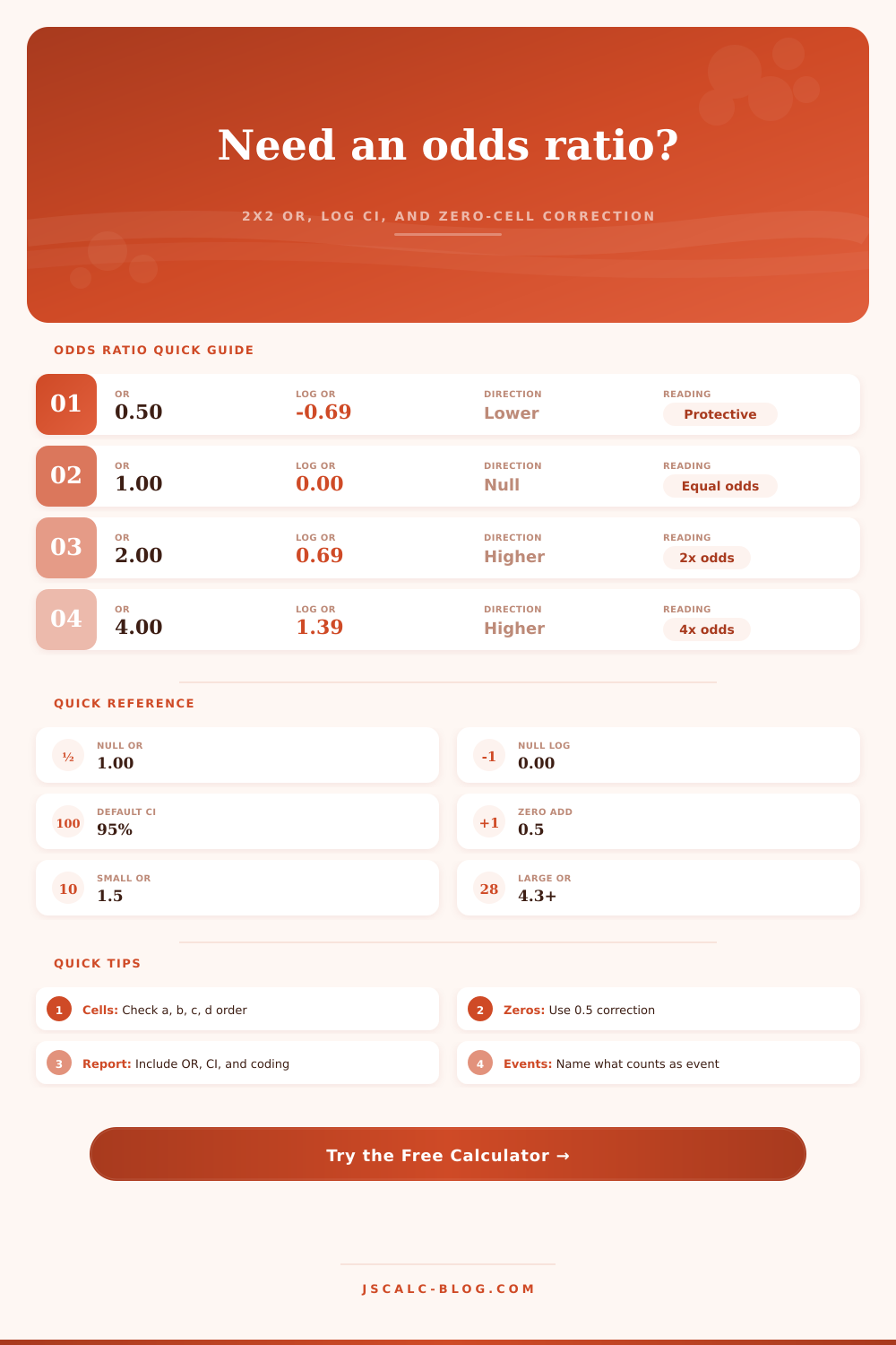
Enter a 2 x 2 table to calculate OR = (a×d)/(b×c), log odds ratio, Wald confidence interval, event rates, and the optional Haldane-Anscombe 0.5 correction for zero cells.
🎯Named 2 x 2 Presets
🧮Odds Ratio Inputs
The formula still uses a, b, c, d exactly as shown below.
CI uses ln(OR) plus or minus z times the log standard error.
Haldane-Anscombe correction stabilizes OR when a cell is zero.
Coding affects wording; it does not change the OR formula.
Top-left cell: event count in the exposed or first group.
Top-right cell: non-event count in the exposed or first group.
Bottom-left cell: event count in the control or comparison group.
Bottom-right cell: non-event count in the control or comparison group.
🔢Current 2 x 2 Snapshot
📐Formula Breakdown
📋Preset Comparison Grid
| Scenario | a | b | c | d | Approx OR | Typical Reading |
|---|---|---|---|---|---|---|
| Trial benefit | 42 | 158 | 24 | 176 | 1.95 | Row 1 has higher desired-event odds |
| Adverse event | 18 | 282 | 10 | 290 | 1.85 | Adverse odds are higher in row 1 |
| Case-control exposure | 86 | 114 | 58 | 142 | 1.85 | Exposure odds higher among cases |
| A/B signup lift | 310 | 1690 | 250 | 1750 | 1.28 | Modest conversion odds lift |
| Screening positive | 72 | 28 | 45 | 155 | 8.86 | Strong positive-classification odds |
| Rare event zero cell | 0 | 80 | 5 | 75 | 0.09* | Correction prevents infinite math |
| Protective exposure | 12 | 188 | 30 | 170 | 0.36 | Row 1 has lower event odds |
| Quality defect audit | 7 | 493 | 19 | 481 | 0.36 | Lower defect odds in row 1 |
| Large cohort check | 1260 | 8740 | 980 | 9020 | 1.33 | Stable estimate with narrow CI |
🧭Interpretation Reference
| OR Range | Log OR Range | Direction | Magnitude Cue | Plain Reading |
|---|---|---|---|---|
| 0.00 to 0.33 | -1.10 or less | Lower odds | Large protective | Row 1 event odds are much lower than row 2 |
| 0.34 to 0.66 | -1.08 to -0.42 | Lower odds | Moderate lower | Row 1 event odds are clearly lower |
| 0.67 to 1.49 | -0.40 to 0.40 | Near null | Small or unclear | Odds are not far from equal |
| 1.50 to 2.49 | 0.41 to 0.91 | Higher odds | Small to moderate | Row 1 has meaningfully higher odds |
| 2.50 to 4.29 | 0.92 to 1.45 | Higher odds | Moderate higher | Row 1 odds are several times row 2 odds |
| 4.30 or more | 1.46 or more | Higher odds | Large higher | Check coding and cell counts carefully |
🔍Confidence and Method Table
| Choice | z Critical | Interval Width | Use When | Reminder |
|---|---|---|---|---|
| 90% CI | 1.645 | Narrowest | Exploratory summaries | Less conservative than 95% |
| 95% CI | 1.960 | Standard | Most reports and abstracts | Still an approximate Wald interval |
| 98% CI | 2.326 | Wider | Stricter screening | Needs enough information in all cells |
| 99% CI | 2.576 | Widest | High-confidence summaries | Can be very wide for rare events |
| Auto 0.5 | Same z | Finite | Any one cell is zero | Adds 0.5 to all four cells |
| No correction | Same z | Exact counts | All cells are positive | Zero cells create infinite estimates |
🧪Odds Ratio vs Nearby Measures
| Measure | Formula Core | Null | What It Compares | Best Use | Main Caution |
|---|---|---|---|---|---|
| Odds ratio | (a/b) / (c/d) | 1 | Odds of event | Case-control and logistic models | Can look larger than risk ratio |
| Log OR | ln(OR) | 0 | Symmetric odds scale | Confidence intervals and models | Must exponentiate for OR reading |
| Risk ratio | [a/(a+b)] / [c/(c+d)] | 1 | Event probabilities | Cohort and trial summaries | Needs row totals to represent risk |
| Risk difference | p1 - p0 | 0 | Absolute event rates | Practical impact statements | Does not show relative strength |
| Diagnostic odds | LR+ / LR- | 1 | Test discrimination | Diagnostic accuracy | Harder to explain directly |
| Phi coefficient | ad - bc scaled | 0 | Binary association | Balanced 2 x 2 association | Sensitive to margins |
💡Practical Odds Ratio Tips
If you’ve read political polling reports or articles on health studies, or been subjected to tech company’s A/B tests, then you know what an odds ratio is. But this seemingly innocent-looking number hides some pretty hefty concept behind it. It sounds similar to a risk ratio, so maybe that’s how you interpret it, right? Wrong. To interpret study results, you must be clear about the difference between odds and probability. Misinterpreting one for the other can lead you to think something is twice as good or bad when it is actualy just half again as likely.
If you have four cell counts to plug into that thing, the calculator does all the work for you. All you have to do is understand what each number corresponds with. Whatever numbers correspond to “exposed” or “treated,” those go at the top. Whatever numbers correspond to “control” or “comparison” (i.e., the group that wasn’t treated), those goes below them. The first column represents the number of things that happened. This can be whatever you want to consider an event. The second column represents everything else.
How to Use an Odds Ratio Calculator
Switch the orientation of these rows and columns and you flip the whole output upside down. What was an odds ratio of 2 now becomes an odds ratio of 0.5. It is the same relationship, just seen in reverse. That’s why most folks forget the easy part: inverting the results.
For example, think about a clinical trial to test whether a new vaccine works. You give some people the drug and others a placebo, then count who got sick. Plug numbers into this thing. The tool figures out that cross-product ratio. It multiplies all the cells along the diagonals, then divides them by each other. Voila. That’s the engine.
You have your answer: How do the odds of getting sick differ between the two groups? One implies no difference at all. The odds are identical. Anything greater than one implies higher chances in the first group. An amount less than one means lower chances. Magnitude does not.
But be sure to note the confidence interval. Your sample only gives you a point estimate. That’s just a guess. The confidence interval informs you about how good of a guess it was. For this math, the calculator uses log scale. Because odds ratios skew, their distribution isn’t symmetric. Taking the natural log transforms the distribution into something more normal. From there we can compute standard error. The tool then raises the limits back to original scale for you. What you end up with is a range that looks familiar. And if that range contains one, then result is statistically insignificant. You don’t have enough evidence to say an effect exists. It’s too noisy in the data to know.
Zero cells create a mathematical disaster When there are no cells (i.e., when nobody in the control group became ill), then you have a mathematical disaster. The denominator goes to zero. The odds ratio shoots to infinity. The math fails. That’s common with small trials or other situations involving rare events.
What does the calculator do? It corrects for continuity. Specifically, it increases each cell by half of a unit. This is called the Haldane-Anscombe correction. It’s a practical solution. It makes the estimate finite, and closes up the confidence interval. It isn’t a perfect solution; it introduces some tiny bit of bias. But still, it’s preferable to getting no result at all. Always note if you’ve made this correction.
The odds ratio isn’t the same thing as a risk ratio. A risk ratio compares the raw probabilities. That’s simpler to convey to non-statisticians. When an event is rare (e.g., if 1% of people become ill), then an odds ratio will be close to a risk ratio. The two numbers will be similar. The numbers converge. But when an event becomes common (say, 50% of the public contracts this illness) the odds ratio inflates the magnitude. It makes it appear larger than it truly is. Some researchers like to report risk ratios for that reason. Other researchers cling to odds ratios because they’re convenient for modeling. An odds ratio fits snugly in a logistic regression equation. You need the log-odds. The model output the odds ratio.
This shows up when you use the tool’s preset scenarios. Consider a screening test for a rare disease, which can generate a huge odds ratio. This doesn’t imply that the test is worthless. If it has a high enough odds ratio, then a positive test would strongly link to having the condition. Yet the absolute risk may remain quite small. You want to know both numbers. The absolute number tells you how great the impact will be. The relative strength tells you how strongly they are linked. With just half the picture, you can’t make good decisions.
Put it to work. Feed in your numbers. Test your intuition. Examine the difference in the event rate. See how the width of the confidence interval expands with smaller sample sizes. It’s a visual demonstration of statistical power. Small samples create wide nets. Tighten the trap and go large. The numbers don’t lie, but unless you understand what you’re seeing, they will lead you astray. Maintain focus on the confidence interval. Clarify the nature of the event. Those two factors make up correct interpretation of the data. The calculator crunches the numbers. Your job: provide the context.