Normal Curve Calculator: Z-Table Area and Probability

Work the standard normal curve two ways. In Z-Area mode, enter a z-score (or two) and pick left tail, right tail, between, or outside to read the exact area under the curve as a decimal and a percent. In Empirical-Rule mode, enter a mean and sigma to see the 68-95-99.7 ranges and their precise percentages.

📈Choose a Mode

🎯Ready-Made Normal Curve Presets

📝Curve Inputs

Area type to compute

Left and right use z1 only; between and outside use both z-scores.

First z-score (z1)

Standardized value, z = (x minus mu) / sigma.

Second z-score (z2)

Only used for between and outside area types.

Mean mu (Empirical Rule)

Center of the distribution for the 68-95-99.7 ranges.

Standard deviation sigma

One sigma step, must be positive for real ranges.

Area decimal places

Controls rounding on areas and percentages.

Raw score x (optional helper)

In Empirical mode, shows the z-score of this raw value.

Percentile display

Percentile is the cumulative left area times 100.

Area under the curve 0 probability as a decimal

Area as a percent 0% chance of landing in this region

Complementary area 0 the rest of the curve, 1 minus area

Percentile of z 0 cumulative left area of z1

🔢Formula Snapshot

Φ(z)0.5(1 + erf(z/√2))

z(x − mu) / sigma

1σ68.27% inside

2σ95.45% inside

📏Empirical Rule 68-95-99.7

Range	Z-Score Span	Area Inside	Area in Tails	Reads As
mu ± 1 sigma	-1 to 1	68.27%	31.73%	About two thirds
mu ± 2 sigma	-2 to 2	95.45%	4.55%	Almost all
mu ± 3 sigma	-3 to 3	99.73%	0.27%	Nearly everything
mu ± 1.645 sigma	-1.645 to 1.645	90.00%	10.00%	90% interval
mu ± 1.96 sigma	-1.96 to 1.96	95.00%	5.00%	95% interval
mu ± 2.576 sigma	-2.576 to 2.576	99.00%	1.00%	99% interval

📊Common Critical Z-Values

Confidence	Two-Tail z	One-Tail z	Left Area at +z	Typical Use
80%	1.282	0.842	0.9000	Rough interval
90%	1.645	1.282	0.9500	90% CI, 0.05 tail
95%	1.960	1.645	0.9750	95% CI, most common
98%	2.326	2.054	0.9900	Tighter interval
99%	2.576	2.326	0.9950	99% CI, 0.01 tail
99.9%	3.291	3.090	0.9995	Very strict test

⚖One-Tail vs Two-Tail Areas

Z-Score	One-Tail Area	Two-Tail Area	Inside Area	Interpretation
1.00	0.1587	0.3173	0.6827	1 sigma bound
1.282	0.1000	0.2000	0.8000	10% one tail
1.645	0.0500	0.1000	0.9000	5% one tail
1.960	0.0250	0.0500	0.9500	2.5% one tail
2.326	0.0100	0.0200	0.9800	1% one tail
2.576	0.0050	0.0100	0.9900	0.5% one tail

🗃Standard Normal Z-Table Comparison Grid

Z-Score	Cumulative Left Φ(z)	Right Area 1 − Φ(z)	Two-Tail Area	Percentile
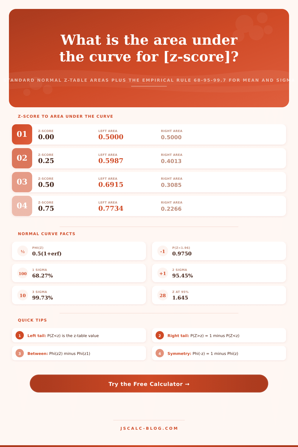
0.00	0.5000	0.5000	1.0000	50.00
0.25	0.5987	0.4013	0.8026	59.87
0.50	0.6915	0.3085	0.6171	69.15
0.75	0.7734	0.2266	0.4533	77.34
1.00	0.8413	0.1587	0.3173	84.13
1.28	0.8997	0.1003	0.2005	89.97
1.645	0.9500	0.0500	0.1000	95.00
1.96	0.9750	0.0250	0.0500	97.50
2.00	0.9772	0.0228	0.0455	97.72
2.576	0.9950	0.0050	0.0100	99.50
3.00	0.9987	0.0013	0.0027	99.87

⚙Formula Breakdown

Φ(z) = 0.5(1 + erf(z/√2))The cumulative area to the left of z. The erf function is evaluated with the Abramowitz and Stegun 7.1.26 approximation, accurate to about seven decimals.

Left tail P(Z < z) = Φ(z)Read straight off a z-table. For z = 1.96 the left area is 0.9750, meaning 97.5% of the curve lies below that z-score.

Right tail P(Z > z) = 1 − Φ(z)The complement of the left tail. For z = 1.96 the right area is 1 − 0.9750 = 0.0250, the classic 2.5% upper tail.

Between P(z1 < Z < z2) = Φ(z2) − Φ(z1)Subtract the smaller cumulative area from the larger. From -1 to 1 that is 0.8413 − 0.1587 = 0.6827, the 68.27% Empirical Rule band.

Outside = 1 − betweenThe two tails combined. Outside -1.96 to 1.96 is 1 − 0.9500 = 0.0500, split as 0.0250 in each tail.

Symmetry Φ(-z) = 1 − Φ(z)The curve is symmetric about zero, so the area left of -1 equals the area right of 1. This is why negative z-tables mirror positive ones.

z = (x − mu) / sigmaStandardize any raw score before lookup. An IQ of 130 with mu = 100 and sigma = 15 gives z = 30 / 15 = 2, sitting at the 97.72nd percentile.

💡Z-Table Reading Tips

Match the tail to the table: A standard z-table almost always gives the cumulative area to the LEFT of z. For a right-tail question, look up the left area and subtract from 1. For a between question, look up both z-scores and subtract the smaller cumulative area from the larger. Sketching the shaded region first stops most sign and direction mistakes.

Use the Empirical Rule as a sanity check: Before trusting a computed area, anchor it to 68-95-99.7. If a z-score is near 1, the inside area should sit close to 68%; near 2 it should be about 95%; near 3, roughly 99.7%. When your calculated number drifts far from these landmarks, you probably shaded the wrong side or misplaced a decimal.

This page contains a calculator that computes probabilities using standard normal curve. We use this as a reference curve because any bell-shaped distribution with mean of 0 and a standard deviation of 1 can be transformed into it. It allow you to compute the area below the curve, i.e., probability. There are two modes available: Empirical-Rule (for rough estimates) and Z-Area (for exact answers).

The area under any probability density curve is always equal to one, or 100% of all possible values. So the slice of area sitting above an interval is what represents the chance a value fall in that range.

How to Use the Z-Score Calculator

Z-tables were invented by statisticians so they didn’t have to do integrals by hand, but this calculator replace paper versions and provides those values live. Just enter your z-score and select a region and get back shaded area as both a percent and a decimal.

Phi of z represent the cumulative left area. Four common areas is covered in the Z-Area mode. The left tail is P(Z z). This is 1, the left area since the entire curve add up to 1. The area between is P(z1 < Z < z2). You take the larger cumulative area and subtract it from smaller area. The outside area are the combined tails, which is 1 minus the between area.

Instead of blindly copying down answers, you see the numbers that’s being substituted and can work through reasoning. How does it calculate? It’s based off error function, from which it gets the cumulative distribution. The error function itself is approximated as a polynomial with an accuracy of seven decimals. Test it: the value for P(Z < 1.96) should of be equal to.9750. This confirms that engine is reliable. The value for the area below Z = 1 (between -1 and 1) are equal to.6827. This again match what the textbook says.

For normally distributed data (the Empirical Rule is your mental model), about 68 percent of the values will falls within one standard deviation from the mean, ~95 percent within two standard deviations from the mean, and ~99.7 percent within three standard deviations. In Empirical-Rule mode, you’ll input the mean and standard deviation, then recieve an exact range of values associated with that band. This is instead of rounded percentages such as 68, 95, or 99.7.

To turn real numbers into z-scores you use this equation: z = (x… Mu) / sigma Empirical-Rule mode let you input a raw number to obtain both the percentile and the corresponding z-score for that number. For instance, if we plug in an IQ score of 130, which has a mean of 100 and a standard deviation of 15, we find out it have a z-score of 2, which is at the 97.72nd percentile. In other words, it’s above nearly all score. The tool do this standardization automatically in Empirical-Rule mode.

The calculator provides critical z-value at various confidence levels (tables are shown below). Notice that 1.96 is based on the 95 percent level while 1.645 is based on the 90 percent. Begin by plugging in an initial example. Adjust the inputs as needed based off your specific situation. Always draw in the area you wish to shade first. Then read off of the number. As a final check, apply the Empirical Rule and make sure your answer makes sense. If it is way outside where you expect things to be, then perhaps you have made a decimal mistake or shaded incorrect side.

For analysts and students alike, this is a handy tool to convert z-scores into plain old shaded areas very fast.