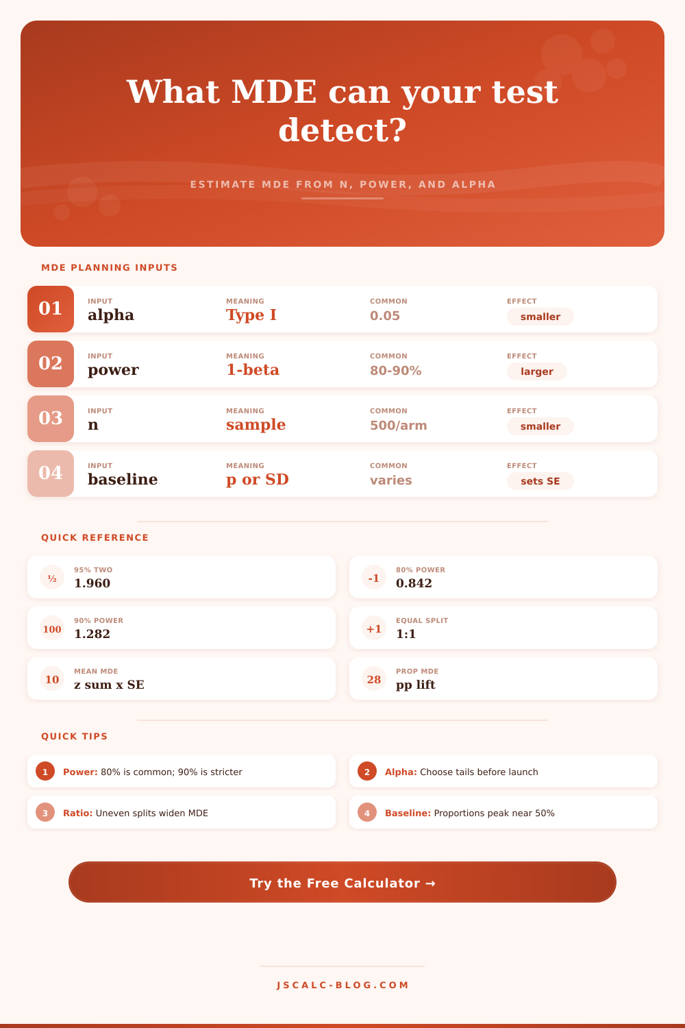
Minimum Detectable Effect Calculator

Estimate the smallest effect your design can reliably detect. Switch between continuous means and binary proportions, then enter sample size, alpha, power, allocation, standard deviations, or baseline rate to see the MDE and formula steps.

🎯MDE Planning Presets

📝Design Inputs

Outcome type

Means use SD inputs. Proportions use baseline p.

Alternative hypothesis

Two-sided designs use z alpha/2.

Significance level alpha

Lower alpha makes the MDE larger.

Target power

Power = 1 - beta, the detection probability at the MDE.

Group 1 sample size n1

Control, baseline, or reference group count.

Group 2 sample size n2

Treatment, variant, or comparison group count.

Group 1 standard deviation sigma1

Use the planning SD for the reference group.

Group 2 standard deviation sigma2

Use the planning SD for the comparison group.

Minimum detectable effect 0 outcome units

Detectable endpoint 0 comparison value at MDE

Standard error 0 before z multiplier

Standardized effect 0 Cohen d or h

🔢Current Design Snapshot

1.960z alpha

0.842z beta

1.00n2 / n1

10000total n

⚙Formula Breakdown

Means MDEdelta = (zα + zβ) x sqrt(sigma1²/n1 + sigma2²/n2). This is the standard normal planning formula for two independent means.

Proportion MDEApproximate MDE = (zα + zβ) x sqrt(p(1 - p)(1/n1 + 1/n2)). The calculator reports it as percentage points from the baseline p.

Critical valueFor two-sided tests, zα = inverse normal(1 - alpha / 2). For one-sided tests, zα = inverse normal(1 - alpha).

Power valuezβ = inverse normal(power). Common values are 0.842 for 80% power, 1.282 for 90% power, and 1.645 for 95% power.

Allocation effectThe calculator uses the entered n1 and n2 directly. Unequal group sizes increase the standard error when the smaller group becomes thin.

Power checkFor proportions, the headline MDE uses the common baseline-variance approximation and then checks achieved power with the alternative endpoint variance.

📊Z Values and Planning Choices

Setting	Alpha or Beta	Two-Sided z	One-Sided z	Power z	MDE Impact
90% confidence	alpha 0.10	1.645	1.282	varies	Smaller MDE
95% confidence	alpha 0.05	1.960	1.645	varies	Standard default
99% confidence	alpha 0.01	2.576	2.326	varies	Larger MDE
80% power	beta 0.20	same alpha	same alpha	0.842	Common screen
90% power	beta 0.10	same alpha	same alpha	1.282	Stricter plan
95% power	beta 0.05	same alpha	same alpha	1.645	Largest MDE

🧪Baseline Proportion Reference

Baseline p	p(1 - p)	Relative Variance	Where Seen	Planning Note
1%	0.0099	Low	Rare events	Normal check may be needed
5%	0.0475	Moderate	Defects, clicks	Small pp lifts need large n
10%	0.0900	Higher	Conversion tests	Common product baseline
25%	0.1875	High	Adoption rates	MDE grows near the middle
50%	0.2500	Highest	Survey shares	Maximum binomial variance
75%	0.1875	High	Retention rates	Same variance as 25%
90%	0.0900	Higher	Pass rates	Mirror of 10%

⚖Allocation Ratio Reference

n2 / n1	Group 2 Share	SE Pattern	When It Fits	Caution
0.25	20%	Much wider	Scarce variant exposure	Thin group drives MDE
0.50	33%	Wider	Limited treatment capacity	Total n often rises
1.00	50%	Most efficient	Equal cost observations	Best default
1.50	60%	Slightly wider	More variant traffic	Usually acceptable
2.00	67%	Wider	Rollout preference	Control gets thin
4.00	80%	Much wider	Rare control plans	Check total n carefully

🔍MDE Scenario Comparison Grid

Scenario	Outcome	n1	n2	Input 1	Input 2	Alpha	Power	Tail	Read
A/B conversion	Proportion	5000	5000	10% p	baseline	0.05	80%	Greater	Small lift test
Email click rate	Proportion	12000	12000	4% p	baseline	0.05	90%	Greater	Rare event lift
Defect reduction	Proportion	900	900	8% p	baseline	0.05	90%	Less	Quality drop
Survey support	Proportion	700	700	50% p	baseline	0.05	80%	Two	Highest variance
Blood pressure	Mean	90	90	12 SD	12 SD	0.05	80%	Two	Clinical units
Website latency	Mean	260	260	90 SD	85 SD	0.05	90%	Less	Milliseconds
Test scores	Mean	160	160	9 SD	10 SD	0.05	80%	Two	Scale points
Battery life	Mean	75	75	2.5 SD	2.8 SD	0.05	90%	Two	Hours
Uneven rollout	Proportion	4000	8000	18% p	baseline	0.05	80%	Greater	2:1 split

💡MDE Planning Tips

Use the smallest useful effect: MDE is a planning threshold, not a promise. If your design can only detect a very large lift, a null result will not rule out smaller useful effects.

Keep units straight: For means, sigma and MDE are in the outcome's natural units. For proportions, the calculator reports absolute percentage points from the baseline rate.

Watch imbalance: A 50/50 split is usually most efficient. If one group is much smaller, the standard error grows even when total sample size looks large.

Check assumptions: Normal approximations work best with adequate sample size, independent observations, stable variance, and enough successes and failures for proportion outcomes.

So first: all experiments start with a question about capability rather then outcome. Before you run the test, you want to know what the design can realy see. Too faint? Then the noise swamps the signal, and you get a null result; meaning nothing. The minimum detectable effect answer a practical question. What’s the smallest difference your study could reliably find under these circumstances? In other words: The resolution of your lens. Maybe you have a blurry lens that sees general shape of a big tree, but doesn’t see individual flowers down by the bottom. But you get to choose what that means.

Once you plug in your variance and your sample size, the calculator do all the math for you. So you don’t waste time trying to convert and guess at coefficients. First, you enter in your baseline value. This matter more than you would think. Variance reaches its peak in the middle for proportions. In other words, if you’re measuring something with an even split between two adult-sized sofa (like, say, support for a given political candidate), then you need more respondents because your data’s inherently noisy. On the other hand, if you’re looking at something rarer, like defects, then you see the same effect size with fewer respondents. The page has a nice reference table laying this out. You can see how the math changes based off moving from one percent to, say, fifty.

What Is Minimum Detectable Effect?

There’s another tradeoff here as well: sensitivity vs. Certainty. Alpha means you don’t want false alarms, which is thinking you see something when it is just a ghost. Power means you don’t want to miss something real, like a true signal. People typically sets their power at 80% and their alpha at 5%. It is not a law but a convention. Bump up your power to 90%, and you’re insisting on more evidence. To cross the higher bar you set, you need a louder effect, or a bigger sample size. So the MDE get bigger.

“Everyone pulls the lever of sample size. The more people you have, the smaller the standard error. That makes the MDE tighter. But it’s not linear. To half the detectable effect, you need a sample that’s four times larger. And that’s a brutal bit of geometry, one reason so many tests flop. Without understanding this, teams assume tiny lifts and don’t realize they must gather an army-sized set of data. The tool makes this reality clear in seconds. It translates abstract goals into concrete numbers.”

Another silent power-killer is allocation. Wasting precision by splitting traffic ineffectively sucks. You can’t have half go to the variant and eight-tenths to the control; that’s only going to increase your standard error. That small group will be the bottleneck, it will determine how certain you are. The reason a fifty-fifty split is so efficient isn’t an accident. It perfectly balances each group’s spread. Straying from that mean you need a far bigger overall sample to make up for it.

What the calculator doesn’t do is give you context. The MDE is a stat limit, not a business limit. Does the effect you’re detecting matter? Are you lifting conversion by half a percent and you have a million users? That’s statistically significant, but it won’t pay for the feature. That’s a different question. The MDE answers “what can I find”. It does not answer “what should I care about.

Define the lowest-power effect you could imagine changing your mind about. Then work backwards. Can your current tools finds this? Examine your inputs. Is the necessary sample size impossible to get? Then reduce power or widen your minimum detectable effect. Negotiate with reality. Reality won’t budge; perhaps your design will.

In the end though, the MDE itself is an exercise in humility. It is an acknowledgement that there are things beyond your ability to spot. You need to decide what does and doesn’t matter. Otherwise, a test becomes nothing more than a coin flip with some overhead. It may yield something but you’ll always wonder if that something is worth anything.

Decide ahead of time what the thing is you’re looking for and then let the data do its work. The picture comes into focus. Everything else is simply waiting on the light.