Lead Time Demand Calculator
Calculate average lead time demand from average daily demand and lead time days, then add variable daily demand, lead time distribution, service percentile demand, safety stock, reorder point, and available stock cover.
🎯Lead Time Demand Presets
🧮Demand, Lead Time, And Service Inputs
Profiles set interpretation only; the calculation uses your inputs.
Used for labels, cards, and table output.
Use true daily usage or shipped demand, net of one-time noise.
Measures variable demand around the average daily demand.
Core formula: lead time demand = average daily demand x lead time days.
Enter receipt variability from supplier or lane history.
Adjusts the lead time variability used in percentile demand.
Higher service percentile raises safety stock and reorder point.
Add days between inventory checks for periodic review policies.
Physical usable stock available today.
Supply already committed and expected before the next reorder point.
Subtract stock already promised to other demand.
Reorder and shortage quantities round up to this increment.
Optional order-up-to level after adding review demand and safety stock.
📌Inventory Position Snapshot
📊Planning Profile Comparison Grid
📦Demand And Lead Time Profile Cards
📋Service Level And Percentile Reference
| Target Service Level | Z Value | Percentile Meaning | Typical Use | Inventory Effect |
|---|---|---|---|---|
| 80% | 0.84 | Demand is covered in about 4 of 5 replenishment cycles | Low consequence stockouts | Light safety stock |
| 85% | 1.04 | Moderate service target with limited buffer | Noncritical slow movers | Low to moderate buffer |
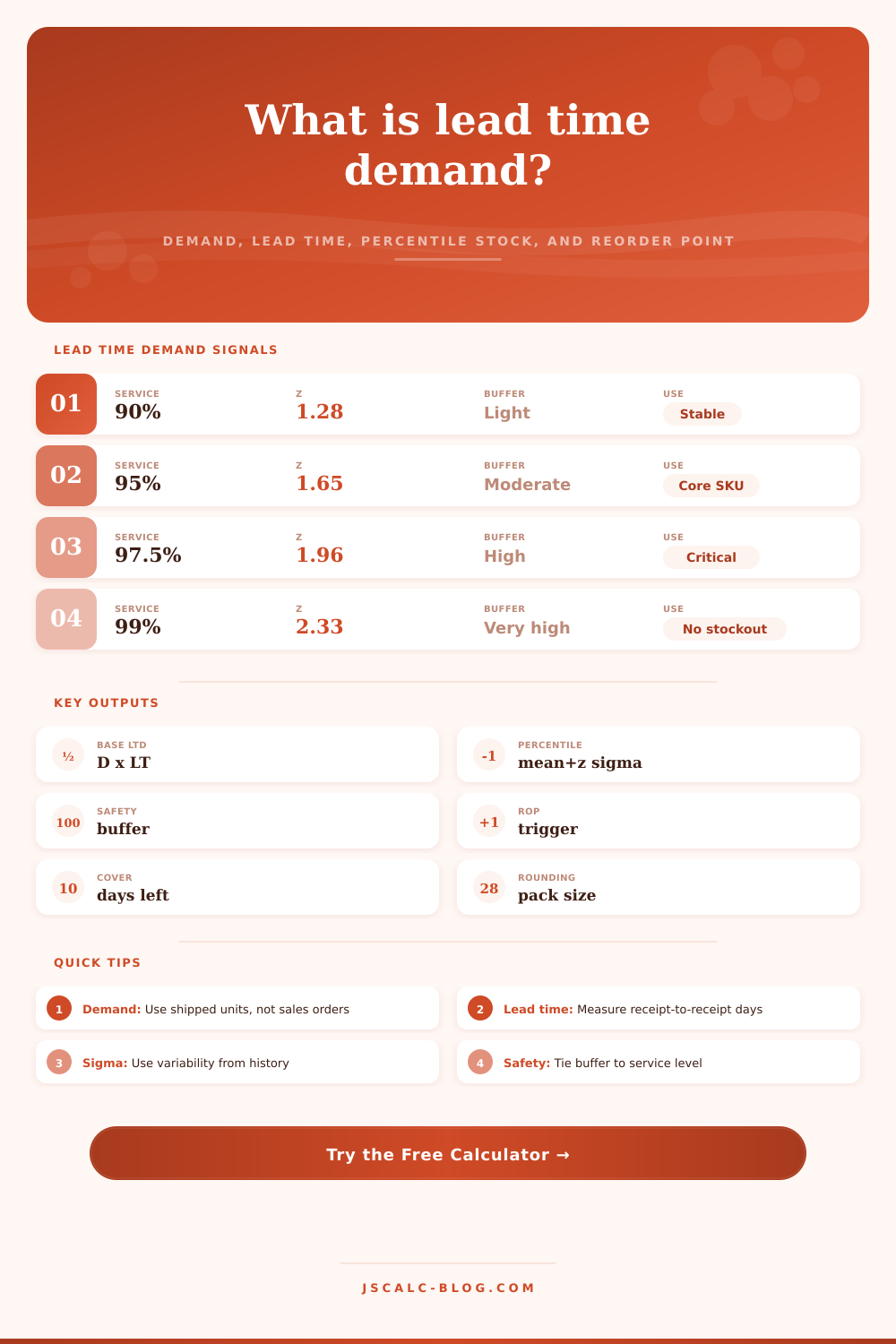
| 90% | 1.28 | Common operating target for stable items | Steady replenishment SKUs | Moderate safety stock |
| 95% | 1.65 | Higher protection against variable demand and lead time | Core items and customer promises | Noticeable safety stock |
| 97.5% | 1.96 | Strong protection for important items | Critical service levels | High buffer |
| 99% | 2.33 | Very high percentile demand coverage | Severe shortage impact | Very high buffer |
🚚Lead Time Distribution Lookup
| Distribution Choice | When It Fits | Calculator Treatment | Planning Watchpoint | Common Data Source |
|---|---|---|---|---|
| Normal variation | Supplier arrivals cluster around the average | Uses entered lead time sigma | Works best with symmetric delay history | Receipt date history |
| Right-tail delays common | Most orders arrive on time, but some arrive late | Raises lead time sigma by 20% | Check whether late receipts are structural | Late PO aging |
| Bounded supplier window | Supplier reliably ships within a narrow window | Reduces lead time sigma by 20% | Do not overstate buffer for disciplined lanes | ASN and dock logs |
| Expedite backup available | Emergency shipments can recover delays | Reduces lead time sigma by 35% | Only use if expedite capacity is realistic | Past expedite records |
| Customs or port delay risk | International or port-constrained supply | Raises lead time sigma by 45% | Delay tails can dominate safety stock | Freight milestone data |
| Shutdown or holiday risk | Supplier or plant calendars create step changes | Raises lead time sigma by 60% | Separate normal cycles from closure cycles | Supplier calendar |
🔍Demand Variability Guide
| Daily Demand CV | Demand Pattern | Safety Stock Read | Forecast Action |
|---|---|---|---|
| 0% to 15% | Very stable movement | Lead time variability may matter more than demand variability | Use recent average and monitor supplier changes |
| 15% to 35% | Typical replenishment variation | Combined sigma gives a balanced buffer | Update demand standard deviation monthly |
| 35% to 60% | Uneven demand or lumpy orders | Percentile demand may materially exceed average LTD | Segment promo, bulk, and recurring demand |
| 60% to 100% | Volatile or intermittent demand | Safety stock becomes sensitive to service level | Consider order-up-to rules and manual review |
| 100%+ | Sporadic demand | Normal approximation may understate extreme spikes | Use scenario review beside the calculator |
📈Service Level Sensitivity Table
| Service Level | Z Value | Percentile Demand | Safety Stock | Reorder Point |
|---|---|---|---|---|
| 95% | 1.65 | 0 | 0 | 0 |
🔢Formula And Method Breakdown
💡Lead Time Demand Tips
Lead time demand is calculated to show the quantity of items you’ll sell before receiving next order. It isn’t just about total sales but also the number of units you will sells between shipments. Simply enter your variability and average into calculator and it’ll crunch numbers without any need to guess about coefficient of variation or standard deviation.
Most folks do it by using Average Lead Time Demand. Multiply average lead time by average daily demand. In our example above (selling 40 per day with an average lead time of 14) you have five hundred and sixty unit. That’s the baseline. That’s assuming everything is perfectly predictable. Exactly forty units sold each day. Exactly 14 days for supplier delivery. If that’s the case there’s no need for safety stock… because you know precisely what you need.
How to Calculate Lead Time Demand
But the world isn’t usually so neat and tidy. Understanding what you’re really measuring is key here. It’s all about exposure. The greater the lead time, the greater window of uncertainty.
Here’s where variability comes into play. One day may be slow while another day will be busy. Weather can cause supply delays. Port congestion might prevent suppliers from shipping goods on schedule. To account for these two types of risks, the calculator first combines lead time variability and demand variability into one standard deviation. Then it multiplies this standard deviation by a Z-value based off your chosen service level. For example, using a service level of ninety-five percent means you’re using a Z-value of 1.65. This ensures you have enough inventory to protect yourself if demand is more than one point six five standard deviations above average.
That’s your safety stock. That’s the cushion which protects you against shock.
There’s also a tradeoff here: between your customers’ happiness vs. Your bank balance. If you want to aim for ninety-nine percent (a pretty good target), then that means you’re going to need a lot more safety stock, and tie up lots of capital in that inventory. If you go for something closer to ninety percent (still not bad) then you’ll risk more stock-outs but keep less inventory on hand. It’s a matter of weighing up what the cost of keeping an extra unit on the shelf would be vs. The cost of losing a dissatisfied customer who leaves empty handed. If it’s critical medical supply, the cost of a stockout is high. If it’s something non-essential, maybe keeping too much of it on the shelf are more costly.
The numbers are only as good as what’s going into them. Garbage in, garbage out. For instance, did you put in sold units rather than shipped units? Did you include cancelled orders? Were there any future dates that didn’t actualy convert? So now you have artificially higher perceived demand. Also, if you measure demand in business days but calculate lead time in calendar days, you’re screwed.
Your lead time should come from when you place an order until it’s usable on the shelf. How long does it take to process it, ship it, and then recieve it? Then how much time to process it? And then how many days for it to ship? All this add up. That’s where most people mess up. They underestimates the receiving delay.
It will also calculate your reorder point. That is your reorder point, which is your safety stock plus your average lead time demand. If you’re checking your inventory occasionally (which you should) then you need to account for how much will be used in the meantime. Otherwise you’ll run dry while waiting for next check. A nice little touch: the calculator rounds these figures to your preferred pack size. Because hey, no ordering half-cases.
Lead Time Demand helps us turn inventory management from a reactive task of guess work, to a proactive approach that actualy works. You’re no longer wondering when to place an order. You know. And all it takes is some honest assumptions regarding variability and clean data. After that, it’s just math.
We aren’t trying to remove all risk. We’re trying to manage it in a smart way. We create a buffer that’s big enough to please our customers but small enough to make our wallet smile. That’s where good operations exist. The truck shows up on-time, the shelves are full, and there’s no scary ghost story ever told. You should of known how important this is.