Hedges G Calculator
Convert two means and standard deviations into Cohen d, the small-sample correction J, Hedges g, an approximate standard error, confidence interval, and practical interpretation.
Independent mode uses pooled standard deviation. Paired mode uses the mean change divided by the SD of paired differences, then applies the same Hedges small-sample correction.
| Step | Independent groups | Paired differences | Interpretation note |
|---|---|---|---|
| Mean contrast | M1 - M2 | Mean time 2 - mean time 1 | The sign tells direction, not quality by itself. |
| Standardizer | Pooled SD from both groups | SD of paired differences | Use the SD that matches the design. |
| Cohen d | (M1 - M2) / pooled SD | Mean change / SD difference | This is the uncorrected effect size. |
| Degrees of freedom | n1 + n2 - 2 | pairs - 1 | Lower df makes J smaller. |
| Hedges g | J times d | J times d | Usually slightly smaller than d. |
| Absolute g | Common label | Plain-language read | Reporting caution |
|---|---|---|---|
| 0.00 to 0.19 | Trivial | Little standardized separation | May still matter at scale or for hard outcomes. |
| 0.20 to 0.49 | Small | Modest but visible effect | Describe direction and context. |
| 0.50 to 0.79 | Medium | Clear separation between means | Check CI width before overclaiming. |
| 0.80 to 1.19 | Large | Strong standardized difference | Look for design or measurement artifacts. |
| 1.20 or more | Very large | Very strong standardized difference | Confirm scales, SDs, and sample handling. |
| Approximation | Formula used here | Best fit | Watch for |
|---|---|---|---|
| Pooled SD | sqrt(((n1 - 1)s1^2 + (n2 - 1)s2^2) / df) | Independent groups with comparable SDs | Large variance imbalance may call for sensitivity checks. |
| J correction | 1 - 3 / (4df - 1) | Small to moderate samples | As df grows, J approaches 1. |
| Independent SE | sqrt((n1+n2)/(n1*n2) + g^2/(2df)) | Quick CI around standardized difference | It is an approximation, not exact meta-analysis software. |
| Paired SE | sqrt(1/n + g^2/(2df)) | Repeated measures summarized by change SD | Requires the SD of paired differences. |
| CI | g plus or minus z times SE | Screening, planning, and reports | Use exact methods for formal inference when needed. |
| Scenario | Design | n pattern | Likely g band | Common use |
|---|---|---|---|---|
| Pilot trial | Independent | 12 vs 12 | Medium | Planning larger study power |
| Classroom test | Independent | 24 vs 26 | Small to medium | Education intervention summary |
| Therapy scale | Independent | 38 vs 35 | Medium | Outcome score comparison |
| Strength plan | Independent | 18 vs 18 | Large | Training response comparison |
| Survey change | Independent | 80 vs 76 | Small | Attitude score difference |
| Lab repeat | Paired | 16 pairs | Medium | Within-person measurement shift |
| Pre-post quiz | Paired | 30 pairs | Large | Learning gain reporting |
| Clinical visit | Paired | 42 pairs | Medium | Symptom scale improvement |
OK, so we did our study. We recruited people into the study. We measured outcomes. We have two number that appear to be different. Is that different enough to matter? Or is that simply result of random noise? Standardized effect sizes provide an answer to that question. They strip out units of measurement and let you know how much overlap there is between two group compared to their own variation. (The most popular standardized effect size is Cohen d, but there’s a hidden issue with it.)
The issue is it’s biased; specifically, it tends to overstate the actual effect in the population, particularly with modest group sizes. This is where Hedges g comes in. It adds a correction factor to Cohen d to take out that upward bias. This provide a more truthful representation of what’s occurring in the world outside of your sample set.
How to Use Hedges g Correctly
Plug those descriptive stats into the calculator above, and it does the rest. Enter the sample size, mean, and standard deviation of each group. If you’re working with independent groups, the calculator also calculates a pooled standard deviation, a key step that creates a common frame of reference from which to compare data. Pooled estimates only work when we assume groups have similar enough variance (otherwise, the denominator will be inaccurate and won’t represent the true population well). The calculators point out this assumption in the references at the bottom. They alert you to check big differences in variances carefully, instead of blindly accepting them as if one number holds true for all.
The magic comes with the J correction. That’s what makes Hedges g different than Cohen d. It has a little bit taken away depending on your degrees of freedom. For large samples it doesn’t really matter. The J factor approaches one, and Hedges g is almost exactly the same as Cohen d. In smaller studies, however, it does make a difference. It lowers the effect slightly. This prevents you from overstating the effects of your intervention. You can see both the unadjusted version (d) and adjusted version (g) side by side on the tool. Being able to compare those two makes it clear just how much your sample size influences your calculation. It brings the abstraction of statistics down to earth… Literally seeing a difference in your findings.
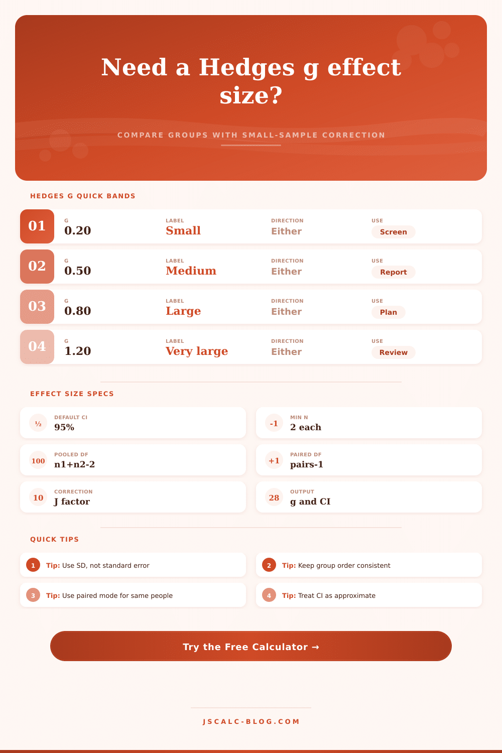
The context comes into play when interpreting how big g is. The page has a reference table laying out convention bands for trivial, small, medium, large, and very large. While these can serve as helpful rules of thumb, they are neither a law of nature nor are they carved-in-stone. What constitutes a “small” effect depends on the context: A small effect from a life-saving medical trial would be much more meaningful then a large effect from a consumer preference survey.
Always compare the effect size to its confidence interval. The calculator will provide an approximate normal distribution interval. This allows you to know the precision of the estimate. If the interval is wide, then there is a lot of uncertainty and it’s possible that the actual effect may differ greatly in the real world. If the interval is narrow, then you have more confidence that what you’re seeing reflects the true effect of the population parameter.
Another key choice is whether to compare paired or independent designs. If your data includes measurements taken twice from the same set of people, you can toggle back-and-forth between these options using this tool. Because it controls for individual differences, paired design typically result in bigger effect sizes. In other words, the standard deviation of the change scores replaces the pooled standard deviation. That alters the denominator, which typically eliminates some of the noise in the calculation. However, that strategy won’t work if your data represents separate groups of people, rather than the same group measured twice. Using the paired option under those circumstances will violate the formula’s assumptions and give you wrong results. The tool tells you to choose appropriately, though ultimately it is up to you to know what kind of data you have.
More transparent reporting makes science better. If we report effect sizes, other researchers can compare our results to those from other studies. This is possible even if they measured something different or used a different scale. Reporting Hedges g is part of building up shared knowledge. Meta-analysts use these reports to pool together studies and reach some larger conclusion. But as the practical tips point out, make sure you report everything. Report the sample size, the mean, the standard deviation, the confidence interval. That way someone else will be able to reproduce your study or add it into their own set of data.
Put less emphasis on statistical significance, which can be manipulated based on sample size, and pay more attention to how it matters in real life: practical significance.
At the end of the day, calculating effect size is humbling. It recognizes that sample represents an imperfect mirror of the population. The small-sample correction reminds us that our data is not perfect. And when you calculate it with Hedges g, you’re going down a more accurate and conservative road. You’re valuing truth over inflating impressions.
This is something you can use in either a power analysis… Or, if you’ve already run a trial, as a way of summing up results in a stable anchor that goes beyond the particular context of your trial. The numbers change, but the principle doesn’t. Accounting for bias means getting a clearer understanding.