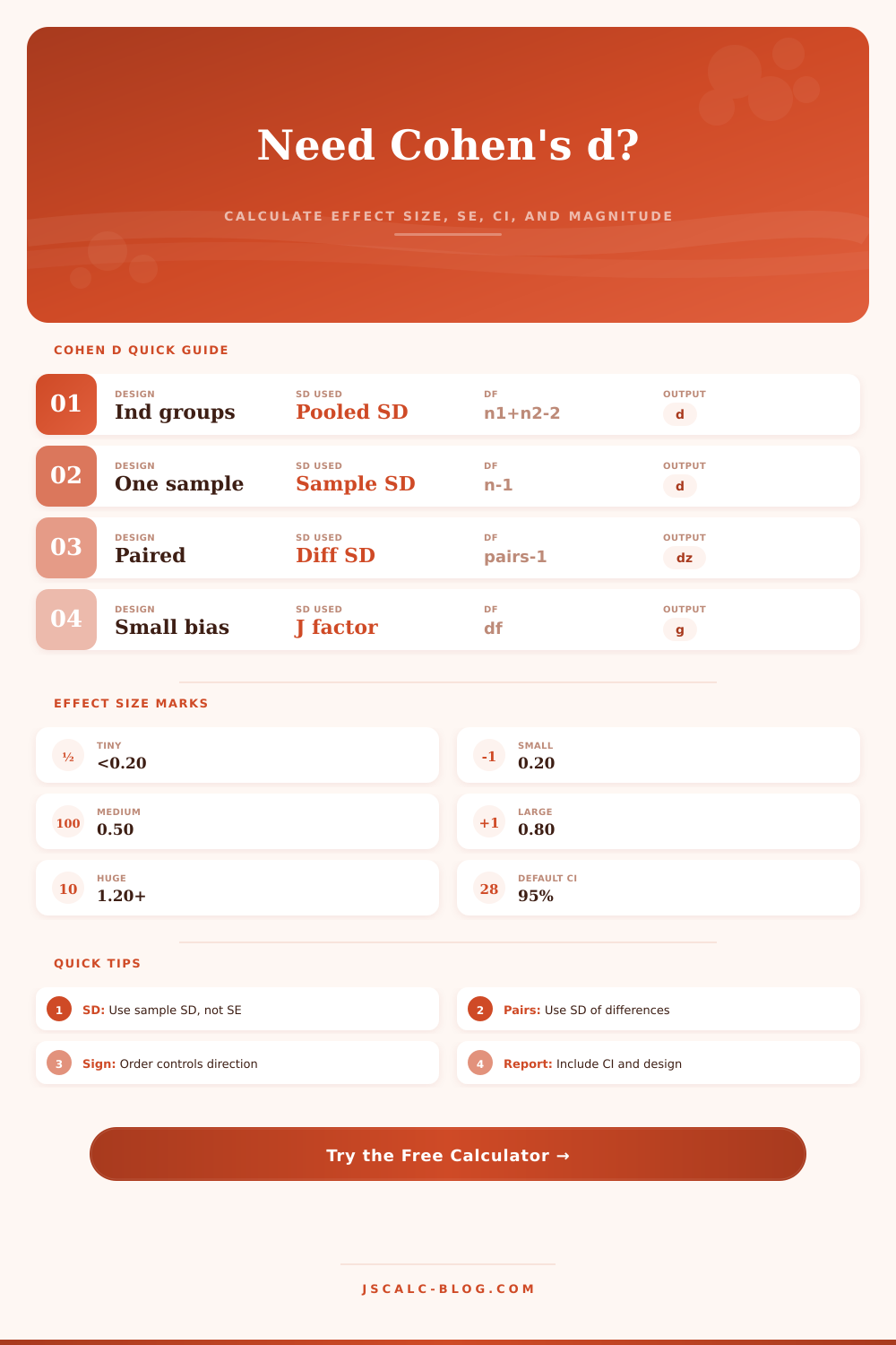
Cohen D Calculator
Estimate standardized mean difference for independent groups, one-sample comparisons, and paired before-after designs. Enter summary statistics to get Cohen's d, Hedges g, approximate standard error, confidence interval, and magnitude interpretation.
🎯Cohen D Presets
📝Effect Size Inputs
Independent groups use both group SDs; paired designs use the SD of within-person differences.
CI is a normal approximation around d using the selected confidence level.
For independent groups, this is the first group mean.
For one-sample mode, this is the benchmark or null mean.
In paired mode, enter the standard deviation of paired differences.
Ignored for one-sample and paired variants, but kept for quick switching.
For one-sample and paired mode, this is the total n.
Used only when the analysis variant is independent groups.
🔢Current Effect Snapshot
📐Formula Breakdown
📊Effect Size Method Comparison
| Variant | Formula | Denominator | Sample Size | Report Label | Main Caution |
|---|---|---|---|---|---|
| Independent groups | (M1 - M2) / sp | Pooled sample SD | n1 and n2 | Cohen's d | Assumes common SD scale |
| Hedges independent | J x d | Pooled sample SD | n1 and n2 | Hedges g | Correction matters most with small n |
| One-sample | (M - benchmark) / s | Sample SD | n | Cohen's d | Benchmark must be meaningful |
| Paired dz | Mean diff / SD diff | Difference SD | Pairs | dz | Not the same as between-group d |
| Glass delta | (M1 - M2) / control SD | Reference group SD | n1 and n2 | Delta | Use when treatment changes variance |
| Standardized response | Mean change / SD change | Change score SD | Pairs | SRM | Similar to paired dz |
| Raw mean difference | M1 - M2 | None | Any | MD | Units differ across measures |
| Correlation r | Association scale | Total variation | n | r | Different meaning from d |
🧪Real Preset Values
| Scenario | Design | Mean 1 | Mean 2 | SD 1 | SD 2 | n1 | n2 | Typical Reading |
|---|---|---|---|---|---|---|---|---|
| Medication symptom trial | Independent | 18.2 | 22.7 | 8.4 | 9.1 | 64 | 61 | Lower scores improved |
| Tutoring exam score study | Independent | 84.1 | 78.3 | 10.2 | 11.5 | 35 | 37 | Moderate academic lift |
| Website task time test | Independent | 42.6 | 51.4 | 18.9 | 21.7 | 82 | 79 | Negative means faster group 1 |
| Therapy before-after | Paired | 11.8 | 16.4 | 7.2 | 0 | 48 | 0 | Symptom reduction |
| Reaction time benchmark | One-sample | 276 | 300 | 52 | 0 | 40 | 0 | Faster than reference |
| Manufacturing torque audit | Independent | 102.8 | 99.6 | 4.4 | 5.8 | 24 | 26 | Quality shift |
| Reading fluency gain | Paired | 132 | 116 | 22 | 0 | 30 | 0 | Instruction gain |
| Employee survey benchmark | One-sample | 4.12 | 3.50 | 0.74 | 0 | 118 | 0 | Above midpoint |
| Plant growth fertilizer | Independent | 18.6 | 15.2 | 5.1 | 4.7 | 20 | 22 | Growth advantage |
📏Magnitude Interpretation Table
| Absolute d | Label | Plain-Language Gap | Overlap Cue | Reporting Note |
|---|---|---|---|---|
| 0 to 0.19 | Very small | Hard to see on the raw scale | Very high overlap | Context may matter more than label |
| 0.20 to 0.49 | Small | Noticeable but modest | High overlap | Can matter at large scale |
| 0.50 to 0.79 | Medium | Clear standardized gap | Moderate overlap | Common benchmark for practical signal |
| 0.80 to 1.19 | Large | Strong difference on the outcome scale | Lower overlap | Check design and measurement quality |
| 1.20 to 1.99 | Very large | Large separation of distributions | Low overlap | Inspect outliers and scale restrictions |
| 2.00 or more | Huge | Extreme standardized gap | Very low overlap | Verify SD, coding, and units |
🔍Confidence Level Reference
| Confidence | Approx z Critical | Width Effect | Best Use | Reminder |
|---|---|---|---|---|
| 90% | 1.645 | Narrowest | Screening or exploratory work | More likely to miss uncertainty |
| 95% | 1.960 | Standard | Most research summaries | Still approximate for d |
| 98% | 2.326 | Wider | Stricter reporting | Needs enough sample size |
| 99% | 2.576 | Widest | High-confidence review | May be very wide with small n |
| Small n | Any level | Unstable | Use Hedges g too | Normal CI is rougher |
| Large n | Any level | More stable | Planning and meta-analysis notes | Magnitude still needs context |
💡Actionable Cohen D Tips
This will allow you to interpret statistics propery.
For instance, you may read that some new teaching method increased scores by 15 points. Sounds good! But then you notice it was a test out of 100, and the control group also increased their score by 10 points. The raw difference here is five. Feels like nothing. But when variation across classes are small, those five points might be a huge jump in performance.
How to Use the Calculator Correctly
Cohen’s d standardizes the difference. It allows you to compare a reading test to a math test. Did a change occur? How large of a change was that in comparison to all the other stuff going on?
Then you input your summary stats into the calculator and it does the work for you. It removes all the pesky calculation mistakes from doing it by hand.
First thing, pick what type of design you have. Two different groups? Then you have two sets of means and standard deviations (e.g., one group on a medication vs. One group is a control group on a placebo). Then it will pool those variances together as a reference baseline. It’s assuming that the variation between groups are about the same. In many cases, this won’t be true and so you’ll want to re-think your design. In general though, pooling the standard deviation produce a strong estimate of spread for practical purposes.
The math changes a bit when you’re doing one-sample comparisons. In this case, you’re testing whether a particular group differs from some known benchmark (e.g., a history target, or the national average). Your denominator is now just the sample’s standard deviation. That’s a subtle but critical difference. Using an incorrect variance estimator will either magnify or shrink size of your effect, which results in overconfidence.
The calculator automatically corrects for degrees of freedom, so that the confidence intervals takes into account the true number of samples and not some idealized population.
The paired design has its oddities too. If you’re measuring the same people before and after an intervention, what you want to know is how much they changed. So you need the standard deviation of the differences. Do not use standard deviations from the separate pre and post measures. Many people make this mistake. As a consequence, you’ll typically underestimate the effect size if you compute it using the wrong SD. It neglects to take into account that first and second measurements is correlated.
In this mode the tool ask you for the SD of the differences. This keeps you on the right track.
But what do we do with that d value? How do we interpret it? There’s no hard-and-fast rule here. Instead, consider these as guidelines: Small = 0.2, Medium = 0.5, Large = 0.8. That means that a d value of 0.5 in one study would count as “medium” but a d value of 0.05 would be a tiny effect.
Context is everything. Saving the lives of thousands of people could be a tiny effect in a massive public health initiative. But finding a cure for a rare disease in a lab setting could be completely meaningless. The reference table on the page lays this out. And then use your own discretion… Determine whether a medium effect justifies a change in opinion or not.
It even computes something called Hedges’ g. Hedges’ g is a correction factor for reducing bias in small samples. When sample sizes gets really tiny, Cohen’s d tends to exaggerate. Hedges’ g pulls it back down to earth. You’ll notice the difference shrinks a bit. That’s a good thing. Better to be careful, rather then to say there’s a miracle when there is only a small improvement.
The confidence interval and standard error provide a range of plausible values. If that range contain zero, then your result isn’t statistically significant. This remains true, regardless of how large the point estimate appears.
But always examine the assumptions. In most cases that means checking normality and homogeneity of variance.
For well behaved data though, Cohen’s d is still the best measure when you’re trying to communicate impact. It makes you consider size, not just importance. A p-value tells you there is an effect. A d value tells you whether or not it matters.
Leave the arithmetic to the software; let them worry about telling the story with the numbers. Only half the battle is knowing the difference. Half the battle is knowing if that difference is big enough to care about, and you should of checked earlier.