Effect Size Calculator
Compare practical magnitude with Cohen d, Hedges g correction, Glass delta, correlation r, eta squared, odds ratio, and log odds ratio.
Choose the summary statistic available from your study.
Direction affects wording, not the arithmetic.
Mean for the treatment, exposed, or first group.
Mean for the comparison or control group.
Use SD, not standard error.
For Glass delta this is the control SD.
Required for pooled SD and Hedges correction.
Required for pooled SD and Hedges correction.
Cohen d: d = (M1 - M2) / SDpooled, where SDpooled = sqrt(((n1 - 1)s1² + (n2 - 1)s2²) / (n1 + n2 - 2)).
Hedges g: g = J x d, where J = 1 - 3 / (4df - 1) and df = n1 + n2 - 2. This reduces small-sample upward bias.
Glass delta: delta = (M1 - M2) / SDcontrol. Use it when treatment may change variability and the control SD is the preferred standardizer.
Correlation and eta squared: r is already standardized, r² is variance explained, eta² = SSeffect / SStotal, and partial eta² from F is (F x dfeffect) / (F x dfeffect + dferror).
Odds ratio: OR = (a x d) / (b x c), log OR = ln(OR), and its large-sample SE is sqrt(1/a + 1/b + 1/c + 1/d). Zero cells use a 0.5 continuity correction.
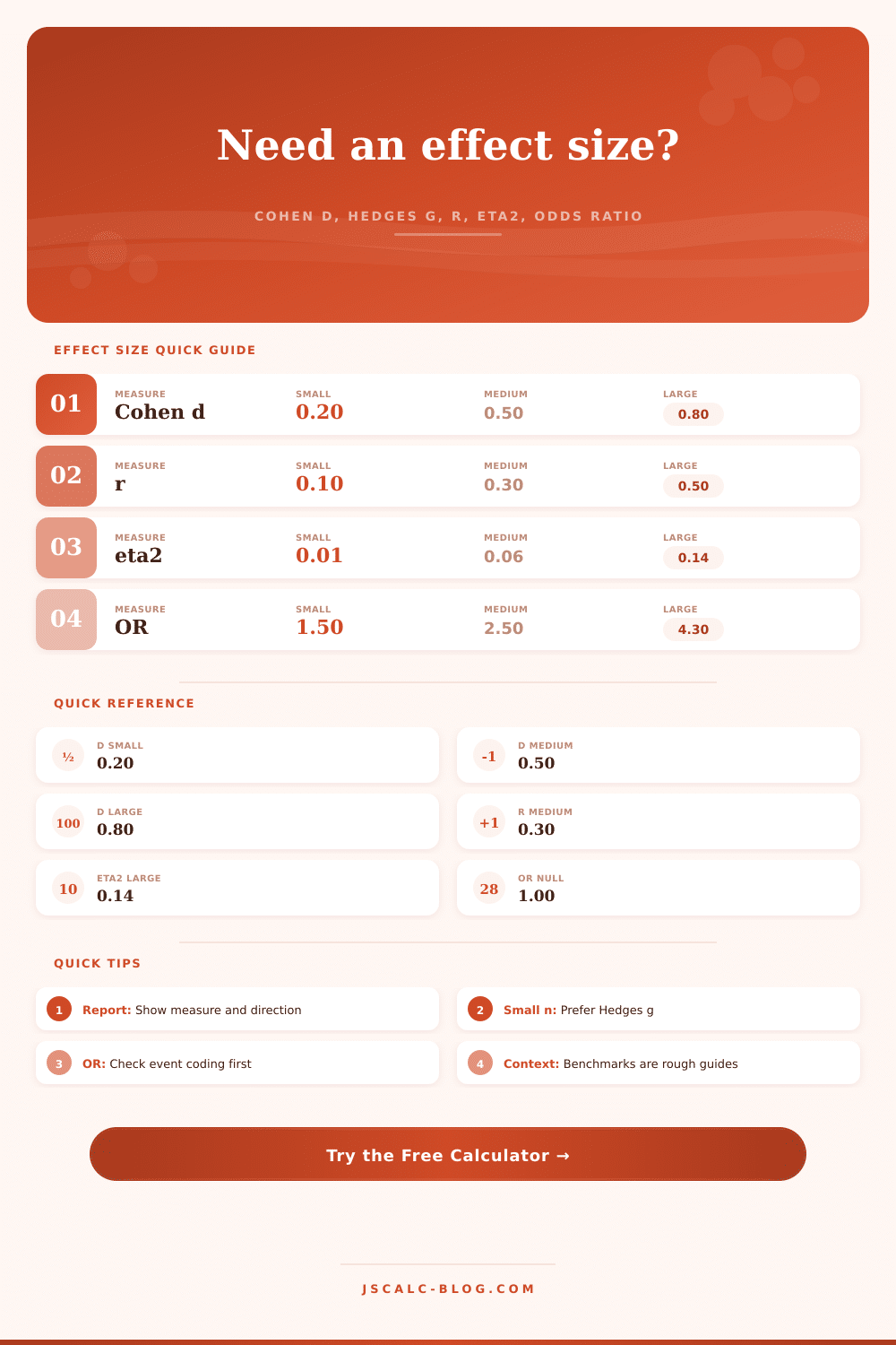
| Measure | Main Inputs | Null Value | Small | Medium | Large | Best Use |
|---|---|---|---|---|---|---|
| Cohen d | Means, SDs, n | 0 | 0.20 | 0.50 | 0.80 | Two independent means with similar variability |
| Hedges g | Means, SDs, n | 0 | 0.20 | 0.50 | 0.80 | Small samples or meta-analysis summaries |
| Glass delta | Means, control SD | 0 | 0.20 | 0.50 | 0.80 | When treatment may alter group variability |
| Correlation r | r and n | 0 | 0.10 | 0.30 | 0.50 | Linear association between two variables |
| r squared | r | 0 | 1% | 9% | 25% | Variance explained by a correlation |
| Eta squared | SS or F with df | 0 | 0.01 | 0.06 | 0.14 | ANOVA proportion of variance explained |
| Odds ratio | 2 x 2 counts | 1 | 1.50 | 2.50 | 4.30 | Binary event odds in two groups |
| Log odds ratio | ln(OR) | 0 | 0.41 | 0.92 | 1.46 | Regression and meta-analysis models |
Standardized Mean Difference Benchmarks
| Absolute d or g | Common Label | Approx r | Overlap Reading |
|---|---|---|---|
| 0.00 to 0.19 | Very small | 0.00 to 0.10 | Groups are highly overlapping |
| 0.20 to 0.49 | Small | 0.10 to 0.24 | Difference is visible but modest |
| 0.50 to 0.79 | Medium | 0.24 to 0.37 | Difference is practically noticeable |
| 0.80 to 1.19 | Large | 0.37 to 0.51 | Group separation is substantial |
| 1.20 or more | Very large | 0.51 or more | Group separation is strong |
Variance and Association Benchmarks
| Measure | Very Small | Small | Medium | Large |
|---|---|---|---|---|
| Correlation r | under 0.10 | 0.10 | 0.30 | 0.50 |
| r squared | under 1% | 1% | 9% | 25% |
| Eta squared | under 0.01 | 0.01 | 0.06 | 0.14 |
| Odds ratio above 1 | under 1.50 | 1.50 | 2.50 | 4.30 |
Odds Ratio Direction Guide
| OR Range | Log OR Range | Direction | Plain Reading |
|---|---|---|---|
| 0.00 to 0.33 | -1.10 or less | Lower odds | Strong protective association if coding is correct |
| 0.34 to 0.66 | -1.08 to -0.42 | Lower odds | Moderate reduction in odds |
| 0.67 to 1.49 | -0.40 to 0.40 | Near null | Odds are not far from equal |
| 1.50 to 2.49 | 0.41 to 0.91 | Higher odds | Small to moderate increase in odds |
| 2.50 to 4.29 | 0.92 to 1.45 | Higher odds | Moderate increase in odds |
| 4.30 or more | 1.46 or more | Higher odds | Large increase in odds |
You run an experiment and the p-value falls below some conventional threshold. Congratulations! Your results is statistically significant. Significance doesn’t tell you how big the effect was, just that the effect are probably non-zero. That’s where effect size comes in: it quantifies the size of outcome.
The calculator up top handles the math for you. You supply the numbers (means, standard deviations, even raw counts), and then there’s the number. Now you know both the size and the likelihood of an effect. Which is better than knowing one without the other.
What is Effect Size?
Cohen’s d is most commonly used tool among researchers. It’s also the one you’re probably most familiar with. To compute it, simply take mean difference between two groups and divide it by standard deviation. The resulting number are standardized, making it possible to compare two sets of data regardless of what type they is.
(Blood pressure? Test scores? It’s no problem. But here’s the catch: When your samples is small, Cohen’s d tend to exaggerate an effect. Enter Hedges g. By including a correction factor for smaller sample, the tool adjust so it’s closer to real effect size. The adjustment isn’t huge, but it could of be the difference between a promising study versus something worth throwing in the trash.
The question is, what do you want to measure regarding standard deviation? Which standard deviation are we talking about? What if there’s an effect on variance after treatment? The standard formula assume equal variances across groups, but if it’s not then you have some noisy results. In those cases, it is better to use Glass delta (the mean difference / control std dev). It maintains the base line while allowing us to understand how large was the change from the norm due to treatment.
Not all measures are created equally. Just because it’s easy to calculate doesn’t make it right for your data. Another way to look at this is through variance and correlation. Eta squared indicates how much of the outcome variance have been explained by the predictor. On its own, an eta squared of 0.14 may sound low, but it represents 14% of the variation explain by the model. That’s nothing to sniff at in social science.
The reference grid on the page contains benchmarks for these figures. Consider those benchmarks a guideline rather than a strict rule. A vital outcome can sometimes have a small but meaningful effect. A variable that is unimportant can have a big one that doesn’t.
The calculator translates between metrics from different scales. That allows you to see that a Cohen’s d of 0.5 and a correlation of 0.3 are both frequently describing the same thing.
The shift is from differences to ratios for binary outcomes. Risk is measured by the odds ratio. If there is no change, the odds ratio equals 1. If it is greater than one, the risk increases. Less than one and its protective. Another number that can be calculated… But not reported as often, is the log odds ratio, which is preferred in regression models since it behaves evenly about zero.
A frequent misunderstanding with an odds ratio is thinking it indicate the direction. What odds are we talking about? Are they the group’s odds or the other groups odds? Is the first group the reference category? Knowing that is crucial. Swapping the categories reverses the odds ratio. What was thought to be a protective effect becomes a risk factor. Clear coding of the inputs in the calculator prevents that kind of error.
The size of the number shows the true strength of the relationship. What’s the difference? Scale is what effect size is all about. Yes or no, That’s what p values are. Effect sizes tells you how much. You can get a tiny effect and still have a significant result. You can have a huge effect, but not have enough power to show it as significant.
What good are they? The full picture comes from reporting both. The tables provides a helpful starting point for setting your own benchmarks. More important than the benchmarks are the stakes of your particular field. In some cases, a tiny change on a test might be fine; in other cases it could be disastrous. Apply the tool to determine how many. Apply your judgment to determine whether it should matter. That is the essence of research.