Exponential Regression Calculator: Fit y = a*b^x, r, R^2

Exponential Regression Calculator

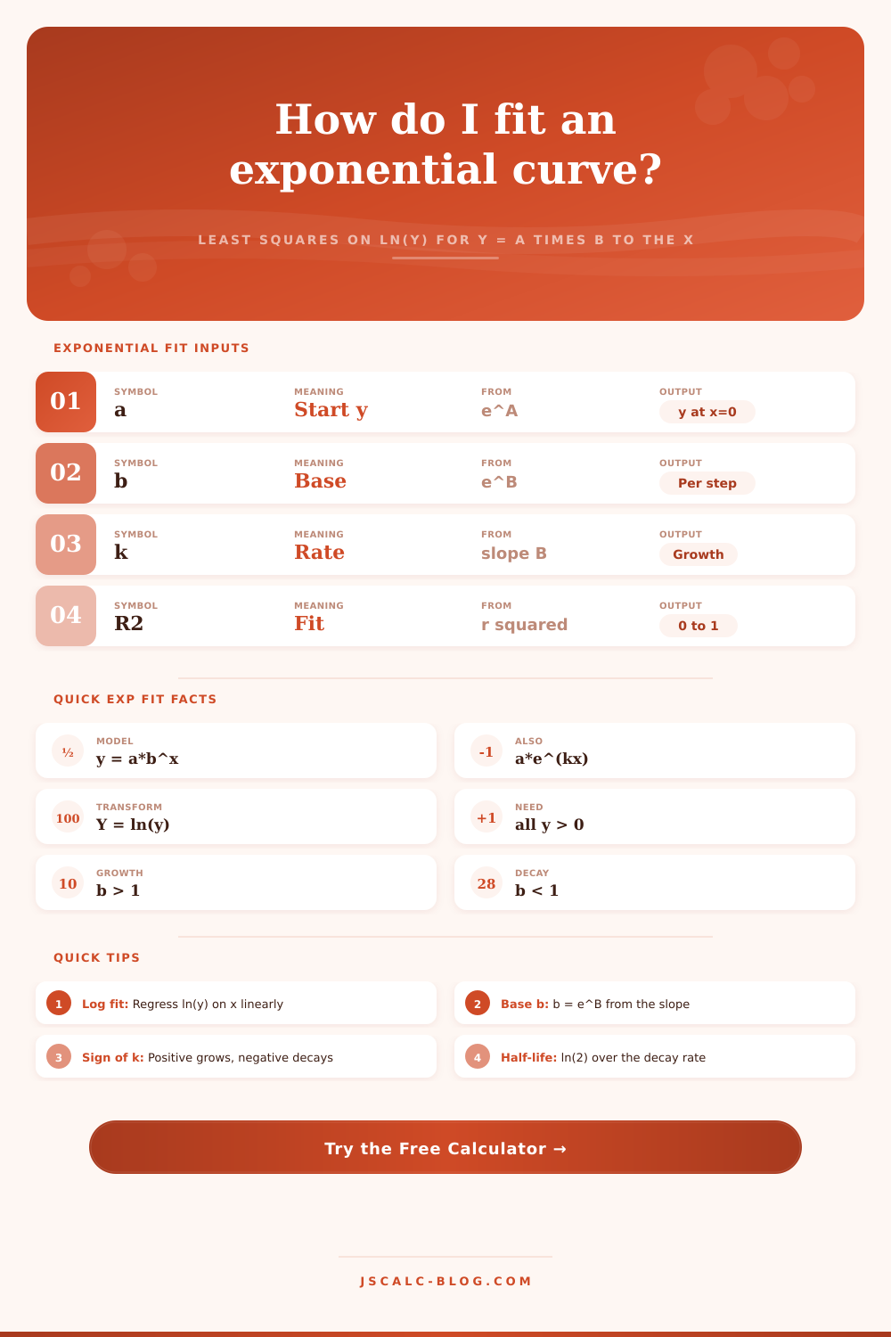
Fit the best exponential curve y = a·b^x (or y = a·e^(kx)) to paired data using least squares on ln(y). Get the coefficient a, base b, growth rate k, correlation r, R-squared, residuals, and a prediction for any x value.

📈Real Data Presets

📝Data and Model Options

X values (independent, comma or space separated)

The predictor. Any real numbers, evenly spaced or not.

Y values (dependent, must all be greater than 0)

ln(y) is taken during the fit, so every y has to be positive.

Model form

Predict y at x =

Estimates y-hat = a · b^x from the fitted curve.

Decimal places

Residual table

Fitted equation y = a·b^x least squares on ln(y)

Coefficient a 0 value of y at x = 0

Base b 0 multiplier per unit x

R-squared 0 fit on the log scale

🔢Model Snapshot

nData points

aCoefficient

bBase

–Trend

🧮Log-Transform Computation Table

x	y	Y = ln(y)	x · Y	x²
Enter X and Y data above to build the least-squares sums.

📋Predicted vs Actual

x	Actual y	y-hat (fit)	Residual	% Error	ln(y) – fit
Residuals appear after the curve is fitted.

⚖Model-Form Reference

Form	Equation	Growth	Decay
Base form	y = a · b^x	b > 1	0 < b < 1
Rate form	y = a · e^(kx)	k > 0	k < 0
Link	b = e^k, k = ln(b)	k = ln(b) > 0	k = ln(b) < 0
Percent	rate = (b – 1) × 100%	positive %	negative %
Doubling	t2 = ln(2) / k	finite & positive	not defined
Half-life	t½ = ln(2) / (–k)	not defined	finite & positive

⚙Least-Squares Formula Breakdown

Step 1 transformReplace each y with Y = ln(y). This turns y = a·b^x into the straight line Y = A + B·x where A = ln(a) and B = ln(b).

Step 2 slope BB = (n·ΣxY – Σx·ΣY) / (n·Σx² – (Σx)²), using the log-values Y = ln(y).

Step 3 intercept AA = (ΣY – B·Σx) / n, the mean of ln(y) minus B times the mean of x.

Step 4 back-transforma = e^A recovers the starting value; b = e^B gives the base. For the rate form the growth constant is k = B.

Step 5 correlationr is the correlation between x and ln(y); the reported R-squared = r² measures fit on the log scale.

Step 6 predictFor any x the fitted estimate is y-hat = a·b^x = a·e^(B·x). Residual = actual y – y-hat.

RequirementEvery y must be greater than 0 because ln(y) is undefined for zero or negative values; such rows are flagged and dropped.

🔎Goodness-of-Fit Interpretation

R-squared (log)	Correlation r	Fit Quality	What It Suggests
0.99 to 1.00	±0.995 up	Excellent	Data is almost perfectly exponential
0.90 to 0.99	±0.95 up	Strong	Exponential model explains most variation
0.70 to 0.90	±0.84 up	Moderate	Trend is exponential but noise is present
0.40 to 0.70	±0.63 up	Weak	Consider power or logistic models too
Below 0.40	near 0	Poor	Little exponential structure in the data

📊Scenario Comparison Grid

Scenario	Typical b	Rate k	Behavior	Doubling / Half-life
Bacteria growth	1.63	+0.49	Fast growth	Doubles ~1.4 steps
Compound interest	1.07	+0.068	Slow growth	Doubles ~10 yr
Population growth	1.025	+0.025	Steady growth	Doubles ~28 yr
Moore's law	1.41	+0.347	Tech doubling	Doubles ~2 yr
Radioactive decay	0.50	–0.693	Decay	Half-life ~1 step
Drug elimination	0.71	–0.347	Decay	Half-life ~2 hr

💡Exponential Regression Tips

Log-linear trick: Plot ln(y) against x. If the points fall on a straight line, an exponential fit is appropriate and its slope is the growth constant k.

Read the base: b tells you the per-step multiplier. b = 1.5 means y rises 50% each unit of x, while b = 0.8 means it falls 20% each step, a decay.

If that sounds familiar, then you’ve seen an exponential curve before (perhaps in math class?). It’s that thing in finance and biology that seem abstract… until it applies to you. Think about how a virus multiplies, or a view count grows for a video, or interest builds in savings account. The more you start with, the faster it increases. The more money you have, the more interest it will earns. The more people watch, the more they share. That is why we get a J-curve. But the fit isn’t linear; it needs special mathematics.

You don’t have to slog through spreadsheets or log transforms manually, just plug in your variables into box above and let the calculator do all the heavy lifting. Linearizing is key technique. Using ordinary least-squares regression won’t work if you try to fit an exponential curve directly, since error would be disproportionately heavy on the high end of your dataset. To get around that, you apply natural logarithm (ln) to the y-values themselves. On a graph, this converts curvy relationship into a straight line. Why does it work? Because a log transform flattens the curve so that you can simply use basic math to calculate its intercept and slope.

How to Fit an Exponential Curve

The calculator handles this process for you: For each pair of x,y coordinate, it calculates ln(y). Just make sure your y-values is all positive; otherwise you’ll have negative and/or zero values which aren’t defined as logarithms in real math. A lot of folks don’t understand what the output coefficients mean. Basically, a is the starting value at x=0. It’s going to be the y-intercept, which may or may not correspond with your initial data point (depending on how noisy your data are). But it establishes the starting line.

Base b is the multiplier for x. So b > 1 mean growth; b < 1 mean decay. This matters because if you try to predict the future, you need to know this. Small changes in b will result in very different predictions over longer periods of time. Folks tend to think about only the next step (which makes sense) without thinking about how the base value compounds over time.

As the reference table illustrates, growth or decay can be given as a rate, involving the exponential e raised to some power. It can also be given as a form, involving a constant multiplied by some base raised to the power x. These are two different ways of describing the same process. When comparing models across disciplines, keep in mind that biologists tend to work with the rate k whereas economists might favor the percentage change (based off b). That’s just a different way of expressing the same quantity: k = ln(b).

R-squared lets you know what percent of the variability in your logged data is accounted for by the linear relationship. If the exponential model fits well (high R-squared), that doesn’t necessarily mean it will make good predictions if the system undergo a subsequent change. Examine the residuals. What’s the difference between the value you actualy observed, versus what the model predicted? Are there any patterns to the errors, not random scatter? Maybe your model has missed something. For example, maybe growth isn’t linearly exponential, but instead logistic (approaching some ceiling, which the model doesn’t account for).

In the real world, things don’t grow forever. Markets becomes saturated. Populations stabilize. Resources get depleted. The calculator provides the best fit for the data you’ve given it, but it can’t anticipate structural limits or external shocks outside of your dataset. This is all about understanding where those numbers apply in whatever it is you’re doing. Radioactive half-lives? Population growth? Same math.

Transform the curve, then fit a line, then back-transform to arrive at your predictions. What’s important is not just taking the resulting equation on faith, but understanding why the transformation occurs. Follow the numbers. Use your judgement to know when to believe ’em.

Remember, though, regardless of how high the rise may appear initialy, every exponential curve will ultimate bend to reality.