Exponential Moving Average Calculator
Calculate EMA_t = alpha * x_t + (1 - alpha) * EMA_prev for prices, traffic, scores, sensor readings, or any ordered data series.
Load a realistic data series, then adjust period, alpha, seed method, comparison period, and output table length.
EMA result summary
Enter a data series and calculate to see the latest smoothed value.
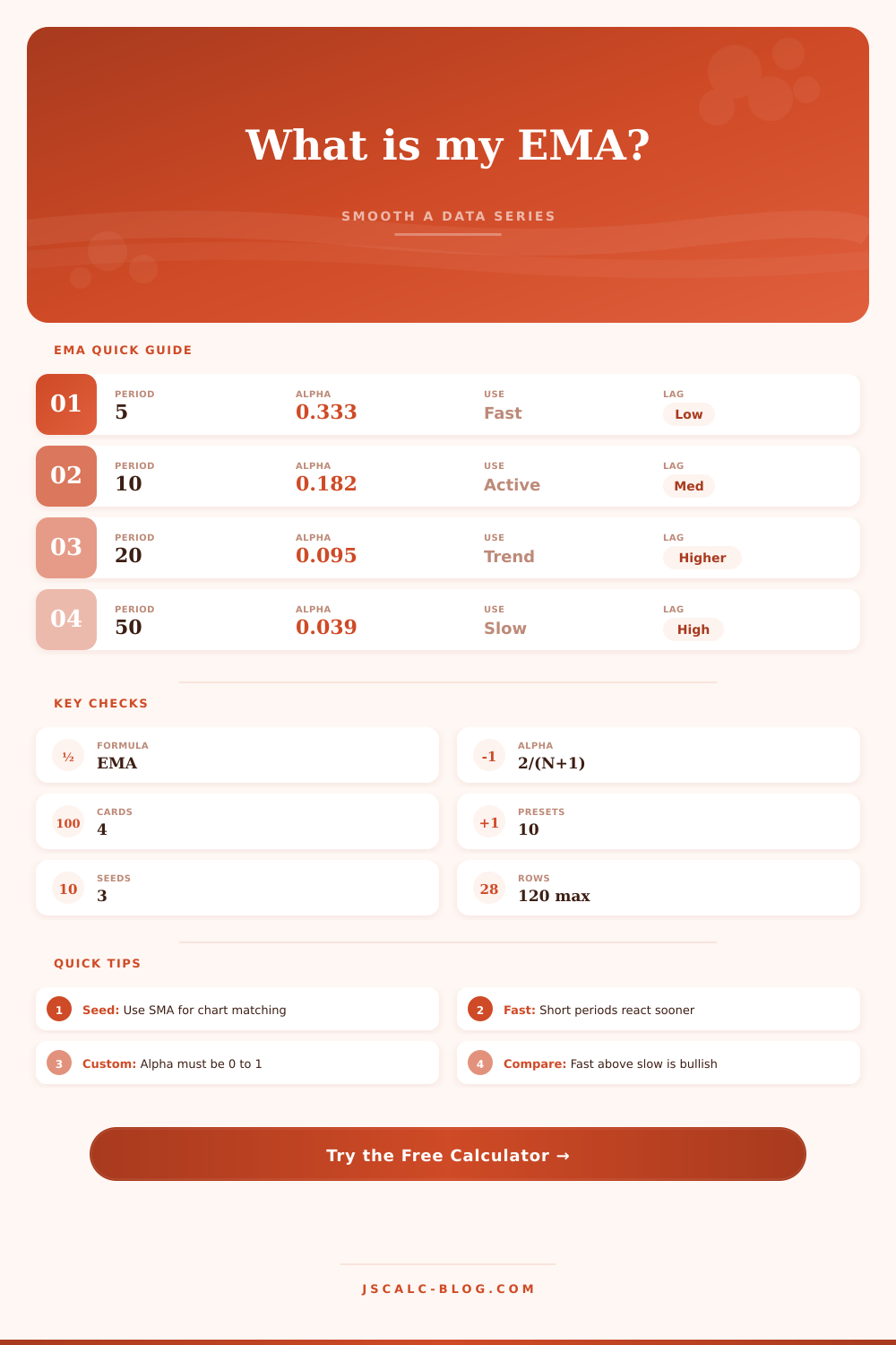
Alpha 0.333. Reacts quickly and can swing on noisy data.
Alpha 0.182. Common for short operational trends.
Alpha 0.095. Balances reaction speed and smoothing.
Alpha 0.039. Useful for broader trend direction.
The latest calculation appears after you run the calculator. SMA seed rows are shown as blank until the first seed is available.
| # | x_t value | Main EMA | Compare EMA | x_t - EMA | Main - compare |
|---|---|---|---|---|---|
| Run the calculator to generate EMA rows. | |||||
| EMA period | Alpha | Old EMA weight | Typical use | Behavior |
|---|---|---|---|---|
| 3 | 0.5000 | 0.5000 | Very fast signal | Responsive, noisy |
| 5 | 0.3333 | 0.6667 | Short trigger | Fast trend shifts |
| 9 | 0.2000 | 0.8000 | Signal line style | Active smoothing |
| 12 | 0.1538 | 0.8462 | Short trend | Moderate lag |
| 20 | 0.0952 | 0.9048 | Baseline trend | Balanced |
| 26 | 0.0741 | 0.9259 | MACD slow side | Smoother |
| 50 | 0.0392 | 0.9608 | Position trend | Slow, stable |
| 200 | 0.0100 | 0.9900 | Long baseline | Very slow |
| Seed method | First EMA value | Best use | Tradeoff |
|---|---|---|---|
| SMA of first period | Average of first N values | Charting platforms and technical indicators | Needs at least N observations |
| First observed value | First x_t value | Streaming data and quick dashboards | Early EMA is influenced by first value |
| Manual starting EMA | User-entered seed | Continuing a prior EMA sequence | Seed must match the previous context |
| Custom alpha | Selected alpha rate | Nonstandard smoothing experiments | Period label becomes descriptive only |
| Formula part | Meaning | Example | Result effect |
|---|---|---|---|
| EMA_t | Current smoothed value | Latest output | Main result |
| alpha * x_t | Weight on current value | 0.0952 * 120 | New data pull |
| (1-alpha) * EMA_prev | Weight on previous EMA | 0.9048 * 116 | Trend memory |
| alpha = 2/(N+1) | Standard smoothing factor | N = 20 | Alpha 0.0952 |
| x_t - EMA_t | Last value gap | Price above EMA | Momentum signal |
The problem with raw data is that it’s too fidgety. There are spikes here and there and dips here and there and pretty soon you can’t find your pattern in all the noise. That’s why we smooth out data. We don’t want to be distracted by every little fluke and instead just want to see big picture, namely, the direction.
An exponential moving average (EMA) are a great way to do that. It remember the past but at the same time gives greater weight to current events. Unlike a plain old moving average, the EMA does not treat 30-day-old data the same as yesterday’s. Instead, the assumption is that what just happened is more important then what happened 30 days ago, so it fades (doesn’t go away) with age by applying some sort of decay factor. As a result, it is faster to respond and hovers closer to the price/value. This makes it attractive to analyst/traders who want to use it to time when to get in/out.
How to Use Exponential Moving Averages
There’s always a catch. In this case, the closer it stays to the price, the more responsive it gets, and that lets more noise through. You have to choose between a smoother signal vs. You get less lag.
You can calculate it by looking at the smoothing factor, which is referred to as alpha. Alpha determines how much weight the current observation gets compared to the previous average. If alpha is high, the EMA will change rapidy because it’s giving more weight to the most recent data point. If alpha is low, then its creating a stable, slow-moving line. The calculator above does this for you, but understanding how the mechanics work make you more confident in the result.
In normal practice, the formula is based off the time period you’re using. So a 50-day EMA has a much lower alpha than a 5-day EMA, meaning the latter will move dramatically from day to day when things get volatile. The former will hardly blink. And neither of them are “wrong.” They simply answer different questions. One is asking: What’s going on here right now? The other is asking: Where is the broad market headed?
Finally, there’s the question of where this all begins: that is, the seed. That’s important because if you’re matching up against a charting service, you’ll probably have to take simple moving average of the beginning data for your own numbers to match what they show. Otherwise the first few points will be off from the rest of the market. For an in-house metric dashboard you might just start with the first point you see or it might not matter. In either case it impacts the early portion of the graph more so than the latter parts, but if you’re backtesting strategies then accuracy here realy counts. You shouldn’ of want to have a bad starting point skew your conclusions about strategy performance.
That’s when most folks do it, just a single period. This forces a limited view. One line shows you the average. You don’t know about momentum. Instead, compare two lines: one slow; one fast. These are called crossovers. If the fast line goes over the slow line, it typically show upward momentum. On the other hand, if it goes under, it indicates a potential downtrend. How far apart they is from each other indicates trend strength. If the gap is wide, then the trend is strong. If the gap is narrow, it shows weakness/consolidation.
On the page, there’s a table that explains this well with how various periods act. There’s nothing magical here but it provides a way to make sense of what would otherwise be chaos.
In the end, though, we’re all seeking clarity. What’s realy going on? How do we separate signal from noise? You aren’t predicting the world with perfect accuracy. You’re just trying to make the noise small enough so you can glimpse reality.
The EMA is about focusing. It makes you pick your historical window. Then once you’ve got that balance dialed-in, you know how to apply it to nearly any time series. You no longer react to each little blip. You begin to see the arc. And that’s worth far more then any individual calculation.