Eta Squared Calculator
Calculate ANOVA eta squared from sums of squares or from an F statistic and degrees of freedom. The calculator returns eta², percent variance explained, Cohen f, and a benchmark interpretation.
🎯Eta Squared Presets
🧮Effect Size Inputs
Use this when your ANOVA table includes effect SS and total SS.
This changes the wording only; the selected formula controls the arithmetic.
SSeffect from the ANOVA row you want to interpret.
Use corrected total SS for standard eta squared.
Optional: used to show partial eta squared context.
Optional for SS mode, required in F mode.
Optional for SS mode, required in F mode.
Enter a benchmark or prior eta² to show the gap.
🔢Current Effect Snapshot
📐Formula Breakdown
📊ANOVA Effect Size Comparison Grid
| Measure | Main Formula | Denominator | Range | Best Use | Common Report | Main Caution |
|---|---|---|---|---|---|---|
| Eta squared | SS_effect / SS_total | Total corrected SS | 0 to 1 | One-way or simple ANOVA variance share | eta² = 0.08 | Can add upward across complex models |
| Partial eta squared | SS_effect / (SS_effect + SS_error) | Effect plus error SS | 0 to 1 | Factorial, repeated, and GLM ANOVA rows | partial eta² = 0.12 | Often larger than standard eta squared |
| F-derived eta squared | Fdf / (Fdf + df_error) | F and df row | 0 to 1 | Published ANOVA tables without sums of squares | eta² from F = 0.09 | Equivalent to partial eta squared from the row |
| Omega squared | Bias-adjusted SS ratio | Total SS plus MS_error | Usually 0 to 1 | Less biased population estimate | omega² = 0.07 | Requires MS_error and full ANOVA details |
| Epsilon squared | Adjusted eta ratio | Total SS | Usually 0 to 1 | Small-sample correction for one-way ANOVA | epsilon² = 0.06 | Less common in software output |
| Cohen f | sqrt(eta² / (1 - eta²)) | Unexplained variance | 0 upward | Power analysis and sample-size planning | f = 0.25 | Depends on which eta squared was used |
📏Eta Squared Magnitude Benchmarks
| Band | Eta Squared Range | Percent Variance | Cohen f Range | Plain Reading | Reporting Note |
|---|---|---|---|---|---|
| Trivial | 0.000 to 0.009 | Under 1% | Under 0.10 | Little variance attributed to the term | May still matter with precise measurement |
| Small | 0.010 to 0.059 | 1% to 5.9% | 0.10 to 0.25 | Detectable but modest effect | Report context and sample size |
| Medium | 0.060 to 0.139 | 6% to 13.9% | 0.25 to 0.40 | Clear variance share for the outcome | Often useful for planning follow-up studies |
| Large | 0.140 to 0.259 | 14% to 25.9% | 0.40 to 0.59 | Strong practical separation | Inspect design, coding, and assumptions |
| Very large | 0.260 to 0.499 | 26% to 49.9% | 0.59 to 1.00 | Dominant term in the model | Check for restricted range or grouped scaling |
| Extreme | 0.500 to 1.000 | 50% to 100% | 1.00 upward | Most variance assigned to one term | Verify SS_total, df, and model specification |
🧪Preset Input Reference
| Preset | Source | Effect Term | Input 1 | Input 2 | Input 3 | df / n Context | Typical Reading |
|---|---|---|---|---|---|---|---|
| Teaching Method ANOVA | SS | Main effect | SS_effect 48 | SS_total 390 | SS_error 342 | df 3, 92 | Medium classroom effect |
| Two-Way Interaction | F | Interaction | F 3.25 | df_effect 2 | df_error 144 | n 150 | Small interaction signal |
| Clinical Group Effect | SS | Main effect | SS_effect 126 | SS_total 812 | SS_error 686 | df 2, 87 | Large clinical difference |
| Process Shift Audit | F | Main effect | F 6.84 | df_effect 4 | df_error 115 | n 120 | Large manufacturing shift |
| Classroom Sections | SS | Main effect | SS_effect 22.5 | SS_total 740 | SS_error 717.5 | df 5, 174 | Small section difference |
| Reaction Task Factor | F | Within factor | F 12.4 | df_effect 1 | df_error 58 | n 60 | Large task factor |
| Repeated Factor Row | F | Within factor | F 4.72 | df_effect 3 | df_error 117 | n 40 | Medium repeated effect |
| Regression Block Test | F | Model block | F 9.18 | df_effect 3 | df_error 196 | n 200 | Medium block effect |
| Large Training Effect | SS | Main effect | SS_effect 210 | SS_total 690 | SS_error 480 | df 1, 78 | Very large training effect |
📋Reporting Checklist Table
| Report Item | What To Include | SS Mode | F Mode | Why It Matters | Example Wording |
|---|---|---|---|---|---|
| Effect label | Name the factor or interaction | Required | Required | Prevents mixing different ANOVA rows | method effect |
| Formula source | State SS or F conversion | SS_effect / SS_total | Fdf / (Fdf + error df) | Readers can tell standard from partial context | computed from SS |
| Degrees freedom | Numerator and denominator df | Helpful | Required | Anchors the ANOVA test row | F(2, 87) |
| Effect size | Eta squared to 2 or 3 decimals | Required | Required | Main variance-share result | eta² = 0.123 |
| Cohen f | Use same eta basis | Optional | Optional | Useful for power planning | f = 0.375 |
| Interpretation | Magnitude plus subject context | Recommended | Recommended | Benchmarks alone are incomplete | medium effect |
💡Two Practical Tips
Finally, after running the analysis, the p-value is looking good. Your experimental group did significantly better then the control. You’re excited to report this! A reviewer requests the effect size. The party has ended in an instant. You know you’ve got a number but is it meaningful? What does it mean?
That’s when eta squared comes into play as your new best friend. It shifts the discussion from “Was there a difference?” to “How large was the actual difference?” In other words, eta squared address the issue of practical significance, something stakeholders may be most concerned with.
Why Use Eta Squared
Eta squared is essentially a variance partitioning statistic, which tell you what proportion of total variation in your data is being accounted for by the factor that you’re investigating. Suppose you have tested three different teaching method; eta squared would tell you what proportion of the variation in student performance are due to the method itself, and not just due to chance (random noise) or variation between individuals.
Six percent? Well, 0.06 indicates that six percent of the variance is explained by the method. Just enter your sums of squares into the calculator above. It does the rest of the work for you, so you don’t have to guess which coefficients to use or if you have the right units.
This post was first published at https://www.noamross.net.
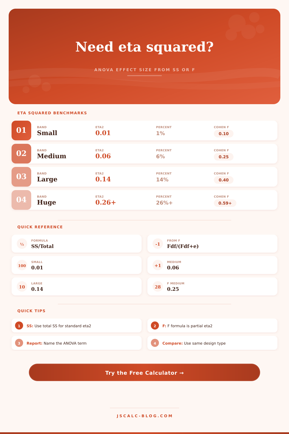
Knowing what denominator to plug into those values isn’t so easy. If it’s a plain ol’ one-way ANOVA, you just take the effect sum of squares and divide it by total corrected sum of squares. The result will cleanly show you how much variance the factor explain. But factorial designs get tricky. With more than one factor in play, you might end up with an unclear standard calculation. Partial eta squared is where a lot of researcher go from there. It separates out the effect by dividing the effect sum of squares by the sum of the effect and error sum of squares.
That’s the approach that the tool on this page follows; it allows you to toggle between the standard eta squared calculation and the F-statistic conversion. The latter is especially helpful if you’re working based off a table in a publication where you don’t have access to the raw sums of squares.
Cohen’s benchmarks are 0.01 for small, 0.06 for medium, and 0.14 for large. Those are useful heuristics, not hard-and-fast rules. What’s “small” in one context could be “clinically very important” in another. What’s “large” in another study could be simply due to a lot of measurement error. There’s a reference table for this on the page, but as always, it depends heavily on context.
How precise were your measures? What was your sample size? With a huge sample size, you can detect small effects that aren’t necessarily practically meaningful at all. That’s why eta squared is useful: It lets you cut through that noise.
A third frequent error I see is people mixing up eta squared and R-squared: Though these two statistics are related, they aren’t the same thing. Eta squared is what you’d use in an ANOVA situation; R-squared is what you’d use in a regression one. And even though they tend to get close in balanced designs, they can differ greatly in unbalanced ones. You’ll reach incorrect conclusions about model fit if you apply wrong statistic. (The calculator gives you an option for calculating Cohen’s f, too, which is handy for conducting a power analysis.)
Finally, it allows you to determine in advance what effect size you would of be able to detect using a particular sample size. This will help you plan your next study.
Reporting these numbers clearly is just as important as calculating them. Are you using partial or standard eta squared? Report it. Do you have any confidence intervals? If so, include them too. By itself, a point estimate can be misleading. Even in small sample size, there’s a lot of variability in the estimate. Acknowledging that uncertainty will make your results appear more believable. It demonstrates that you’re aware of what your data can and cannot tell you.
Ultimately, that’s what effect sizes are: communication. Communication of abstract stats into tangible impact. It communicates whether your audience should act on something. A significant p-value is simply the entry ticket. It’s the performance. And make sure that you’re telling the whole story.