Empirical Rule Calculator
Enter a mean and standard deviation to get the 68-95-99.7 ranges for a normal distribution, plus the z-score of any value, its sigma band, an approximate percentile, and the percent of data between two points.
📌Real Distribution Presets
📝Distribution Inputs
Only relabels the ranges; the math is unit free.
Must be greater than 0 for a valid spread.
z = (x − μ) / σ.
Percent of data between the two bounds via whole-sigma slices.
🔢Formula Snapshot
📊Empirical Rule Percentages
| Interval | Multiplier | % Inside | % Outside | One Tail |
|---|---|---|---|---|
| μ ± 1σ | k = 1 | 68.27% | 31.73% | 15.87% |
| μ ± 2σ | k = 2 | 95.45% | 4.55% | 2.28% |
| μ ± 3σ | k = 3 | 99.73% | 0.27% | 0.135% |
| μ ± 1.96σ | k = 1.96 | 95.00% | 5.00% | 2.50% |
| μ ± 2.58σ | k = 2.58 | 99.00% | 1.00% | 0.50% |
🧩Sigma-Band Slice Breakdown
| Slice (from μ) | Left Side | Right Side | Both Sides | Cumulative |
|---|---|---|---|---|
| 0 to 1σ | 34.13% | 34.13% | 68.27% | 68.27% |
| 1σ to 2σ | 13.59% | 13.59% | 27.18% | 95.45% |
| 2σ to 3σ | 2.14% | 2.14% | 4.28% | 99.73% |
| Beyond 3σ | 0.135% | 0.135% | 0.27% | 100.00% |
📏Z-Score to Band and Percentile
| Value Position | z-score | Band | Approx Percentile | Notes |
|---|---|---|---|---|
| μ − 3σ | −3.0 | 3rd SD | 0.13% | Far low tail |
| μ − 2σ | −2.0 | 2nd SD | 2.28% | Low outlier edge |
| μ − 1σ | −1.0 | 1st SD | 15.87% | Below average |
| μ (mean) | 0.0 | Center | 50.00% | Middle of curve |
| μ + 1σ | +1.0 | 1st SD | 84.13% | Above average |
| μ + 2σ | +2.0 | 2nd SD | 97.72% | High outlier edge |
| μ + 3σ | +3.0 | 3rd SD | 99.87% | Far high tail |
🗂Common Normal Datasets
| Dataset | Mean μ | SD σ | 68% Range | 95% Range | 99.7% Range |
|---|---|---|---|---|---|
| IQ scores | 100 | 15 | 85 to 115 | 70 to 130 | 55 to 145 |
| SAT section | 500 | 100 | 400 to 600 | 300 to 700 | 200 to 800 |
| Adult male height (in) | 70 | 3 | 67 to 73 | 64 to 76 | 61 to 79 |
| Class test grades | 75 | 8 | 67 to 83 | 59 to 91 | 51 to 99 |
| Systolic pressure | 120 | 10 | 110 to 130 | 100 to 140 | 90 to 150 |
| ACT composite | 21 | 5 | 16 to 26 | 11 to 31 | 6 to 36 |
⚙Full Formula Breakdown
💡Empirical Rule Tips
Allow yourself to collect enough data, and you’ll find that it tends to follow what is called the normal distribution, which is the pattern you see with manufactured bolt diameters, human height, or test scores. That is to say, most values tend to bunch up around the mean (average), while fewer values occurs as you approach extreme ends.
Because of this pattern, statisticians has established a set of rules that can help you predict where your data point will fall on the curve. It’s known as the empirical rule. In effect, it takes something that has a lot of random variation and makes it predictable, if you know how to read shape of the curve.
How to Use the Empirical Rule
When you input your standard deviation and mean, the calculator does the work. You no longer have to manually convert or try to guess which coefficient go with what. If you know what those two figures mean, it help you make better use off the output. The mean represent the center of gravity for the set of data. That’s where the curve hits its peak. Standard deviation represents the spread. How closely grouped together are the points centered on the mean? The smaller the number, the closer all value will be to the mean. The larger the number, more spread out they will be.
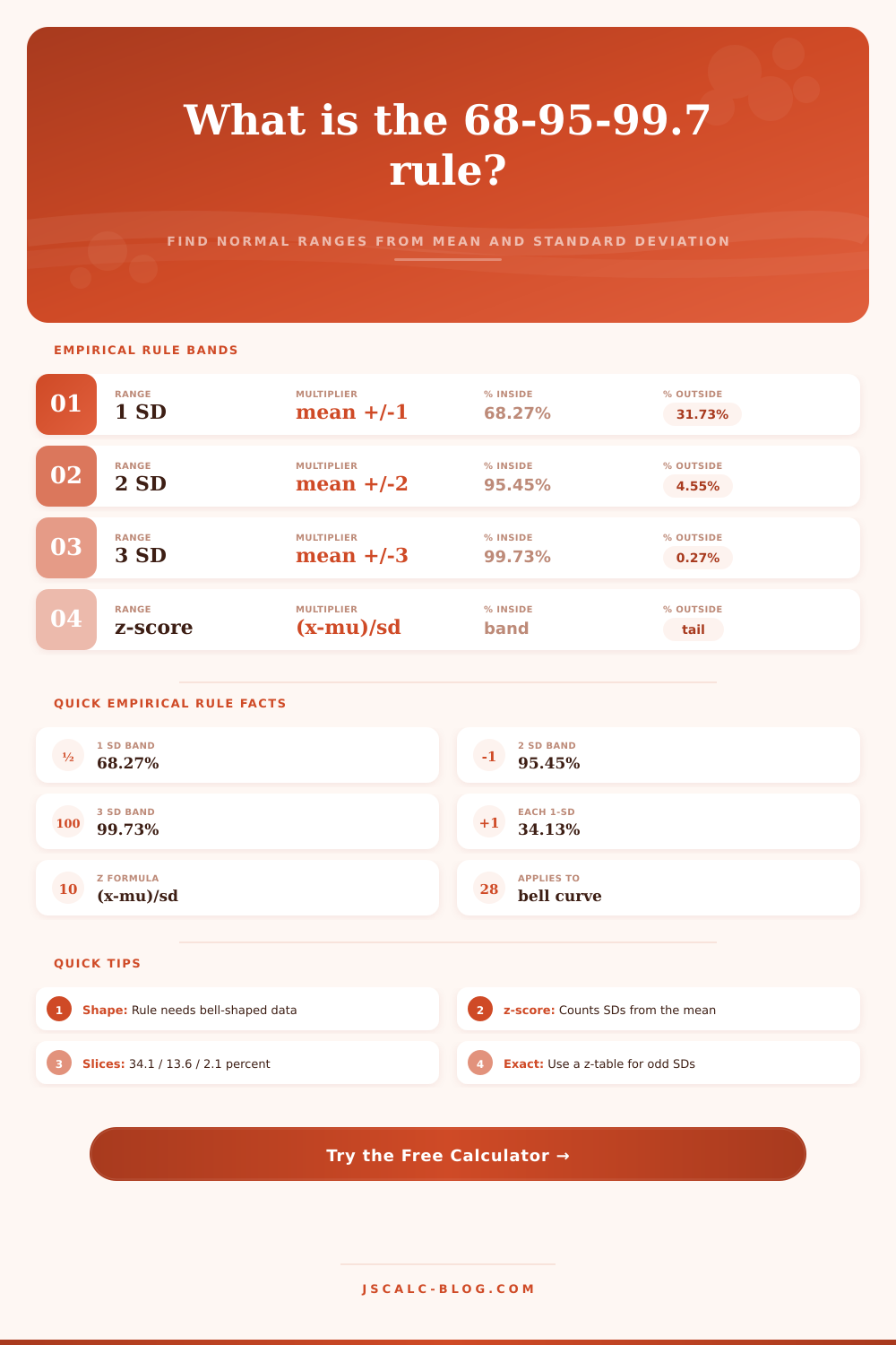
You need both numbers in order to apply the 68-95-99.7 rule: One to define the location, the other to define the shape. What do those numbers mean? They tell you what to plan on. For any normal distribution, approximately 68% of data will be found within one standard deviation of the mean. Expand that to two standard deviations, and you’re capturing around 95%. Extend it out to three, and you gets nearly the full group (99.7%) locked down inside that window.
Those aren’t wild guesses; they’re mathematical certainty when dealing with a symmetric bell curve. Armed with that information, you can quickly assess probabilities without needing to run through complex integrals. You see something two standard deviations removed from the mean? You already know it’s an outlier that shows up maybe four and a half percent of the time. That context is very valuable for assessing risk.
You’ll also frequently see reference to what’s called a z-score. It might sound scary, but it’s simply a kind of ruler. It lets us know by how many standard deviations a given score lie from the average. If I get a z-score of zero, I’m smack dab on the average. A score of plus one? That’s one step up from there, in whatever units your information happens to be measured in. This standardization is why the empirical rule holds true in various areas: two standard deviations from the mean is still the rare top-tier whether we’re talking about blood pressure millimeters or IQ points.
Enter a particular instance into the tool and you’ll get its calculated z-score, allowing you to place it somewhere on the standard normal curve. And on that page, they have a reference table that explains it all at a glance. It lets you look up exactly what percentage is in every band, both inside and out. It’s great if you’re looking for something like “what percentage of kids fell between one standard deviation below the average and two standard deviations above?” You can add them up: what are those pieces? Why, the curve divides itself into predictable chunks on either side! Thirty-four percent of it is the first piece from the middle out. Add another roughly thirteen percent. The last visible slice is just over two percent. So just add up the pieces that apply to you, and there you go.
Here’s the caveat: this applies *only* when your data is normally distributed. Which means if there are two clear peaks in your data, or if it’s severely skewed to either end of the bell curve, all this percentage stuff should of gone out the window. It is a little detail, but it is important nonetheless. Always plot your data on a histogram. Do so before you try any other analysis. If it isn’t symmetric, you’ve got to use a different kind of statistical model.
Remember: the empirical rule assumes balance and symmetry. And when it exists, this is such a powerful way to see the hidden structure inside your numbers.