Confidence Interval for a Difference in Proportions Calculator
Enter successes and sample sizes for two groups to estimate p1 minus p2 with a normal confidence interval, standard error, margin of error, and percent-point bounds.
Load a common two-proportion example, then adjust labels, successes, sample sizes, and confidence level.
| Confidence level | Two-sided z | Effect on interval | Typical use |
|---|---|---|---|
| 80% | 1.282 | Narrowest | Screening estimate |
| 90% | 1.645 | Narrow | Exploratory comparison |
| 95% | 1.960 | Standard | Common reports |
| 97.5% | 2.241 | Wider | Stricter summary |
| 99% | 2.576 | Widest here | High confidence |
| Method | Effect scale | Primary inputs | Best used when | Adjustment style | Watch point |
|---|---|---|---|---|---|
| Wald risk difference | p1 - p2 | x1, n1, x2, n2, z | Large samples with stable rates | Unpooled SE from observed p | Can under-cover near 0 or 1 |
| Wilson / Newcombe | p1 - p2 | Separate Wilson score limits | Better small-to-medium samples | Combines score intervals | Bounds are not symmetric |
| Agresti-Caffo | p1 - p2 | Add one success and one failure | Simple small-sample improvement | Plus-four adjusted proportions | Slightly shrinks extreme rates |
| Miettinen-Nurminen | p1 - p2 | Constrained score calculation | Clinical and formal reporting | Score-based constrained MLE | Usually needs software |
| Relative risk CI | p1 / p2 | Event and non-event counts | Comparing rate multiples | Log-scale standard error | Undefined if p2 is zero |
| Odds ratio CI | Odds1 / odds2 | 2 x 2 table counts | Case-control style summaries | Log odds ratio interval | Harder to read as risk change |
| Exact / unconditional | Usually p1 - p2 | Full 2 x 2 count table | Very sparse or boundary counts | Enumerates possible tables | Can be conservative |
| Scenario | Group 1 | Group 2 | Difference | 95% CI cue |
|---|---|---|---|---|
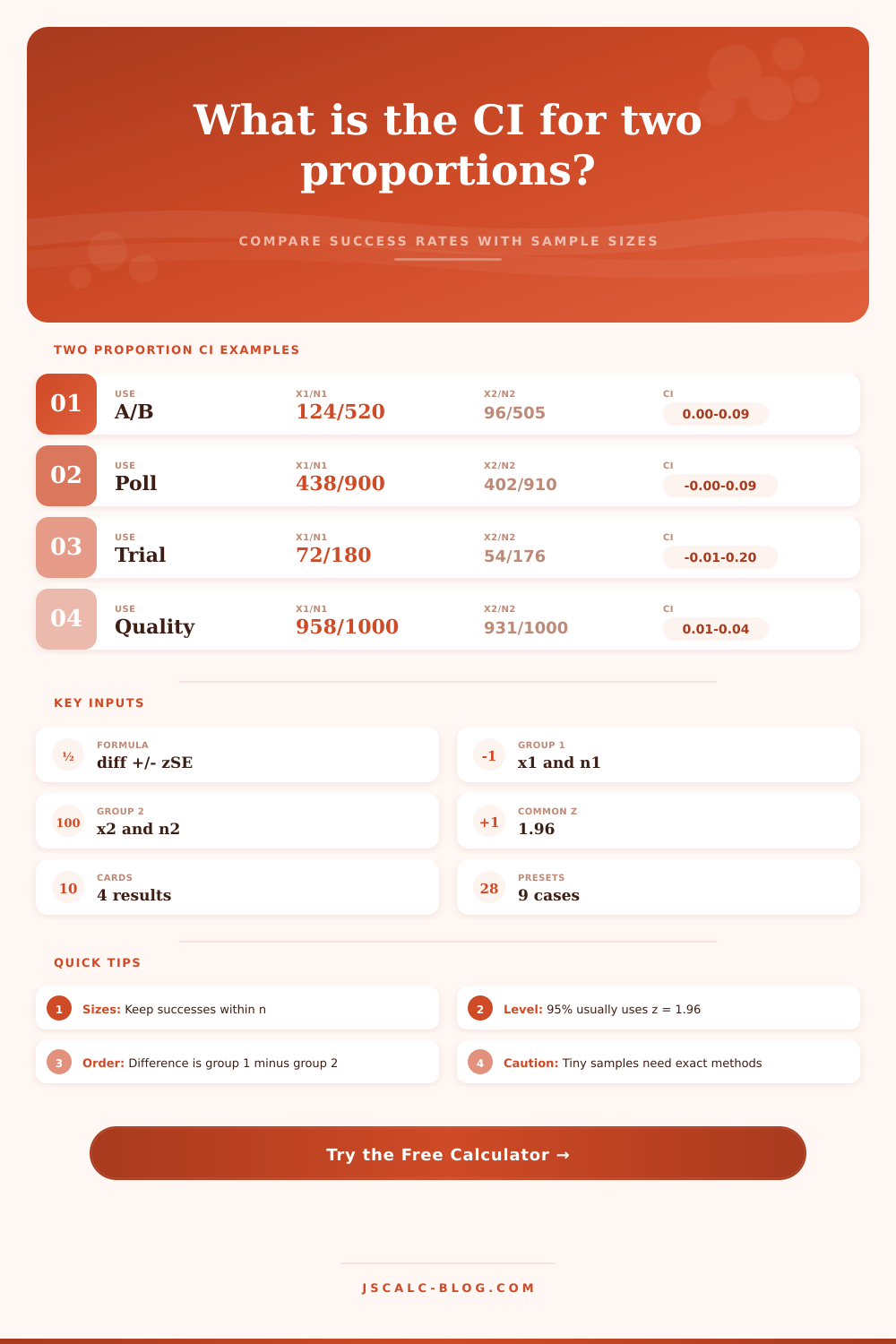
| A/B signup | 124 / 520 | 96 / 505 | +4.84 pp | Small positive |
| Clinical response | 72 / 180 | 54 / 176 | +9.32 pp | May include zero |
| Voter support | 438 / 900 | 402 / 910 | +4.55 pp | Borderline |
| Quality pass | 958 / 1000 | 931 / 1000 | +2.70 pp | Likely positive |
| Email clicks | 212 / 4200 | 178 / 4150 | +0.76 pp | Very narrow scale |
| Graduation rate | 312 / 380 | 287 / 372 | +5.03 pp | Moderate positive |
| Defect reduction | 31 / 1500 | 48 / 1480 | -1.18 pp | Lower defect rate |
Is there a difference between two groups? That’s the question that leads to decisions in public policy, marketing, and medicine. Does a new drug work better then a placebo? Which button; red or blue, gets more clicks? Will a training program boost test scores?
If you’re running an experiment with two group, you have the raw number of successes in each group. But raw numbers is noisy. They tell you only about what happened in your sample. Confidence intervals turns that sample information into a range of values that plausibly reflect actual difference.
How to Compare Two Groups
Once you put in your sample sizes and success counts on the calculator above, it do the math for you. No need to manually calculate critical values and standard error formulas. Simply input the total sample size and number of successes for group one. Do the same for group two.
The tool will determine the sample proportion for each group and calculate difference between groups. Next it creates a range around that difference, we aren’t estimating a single number here; we are estimating a boundary. So if this range contains zero, it means you don’t have a statistically significant difference. And if the whole range is positive, it’s probably safe to assume group one did better then group two. The wider the range, the less certain you can be.
That confidence comes from sample size. Even if two groups has differing success rates, a study of just fifty in each will result in a broad interval. If a study have five thousand people in each group, then resulting interval will be narrow. You can get more precise about the difference.
The normal approximation method is what calculator employs. It’s appropriate for large samples where success rate isn’t close to zero or one. This method assumes a standard error, which is the variation in the differences in proportions when the same study are repeated. A larger standard error lead to wider bounds.
Another trade-off you control is your confidence level. In almost every field, this defaults to 95 percent. So there is roughly a 5 in 100 chance that if you repeated the experiment a hundred times, the interval would miss the true result. (In other words, out of one-hundred experiments, it would catch the correct answer somewhere between ninety-four and a hundred times.) You can change that number around inside the tool.
Raise it to ninety-nine percent, and you’ll be more certain that you’ve got the real thing. However, this comes at the cost of having a wider interval that provides little help with making particular decisions. Drop it down to ninety percent, and you’ll narrow the interval, and know more precisely what the true difference is… But risk being wrong about it.
Here’s how z-scores change with different levels of willingness to err:
A lot of folks misinterpret these results. While they obsess over whether the interval doesn’t include zero, they overlook size of the effect. It may be tiny. Perhaps the new web design increases conversions by half a percentage point. This might well be statistically significant. Perhaps the interval doesn’t include zero, which indicates that there is real change here. But that doesn’t mean it’s worth the expense of implementing. That requires you to consider practical importance. Does the lower end of the interval exceed some number that matters for your bottom line? Is the upper end low enough to eliminate wild speculation?
The calculation alone isn’t everything. It’s also important to understand context. Does the comparison include current standard of care? Is it comparing against a baseline risk? Ten percentage points could mean nothing if the thing being tested is extremely common and everything if it’s rare. It’s up to you to judge. The calculator does the math; you supply the judgment.
Second, you want to make sure your data fits the conditions for which the normal approximation was designed. If you have a small sample size or an extreme success/failure rate then the normal approach may not apply. Score-based intervals or exact methods is preferable in these instances (but more complicated). For the majority of large scale comparisons, however, the standard approach hold up just fine.
In the end, though, this thing enables you to go from wondering to knowing. It moves from “did it work?” to “it was probably a little bit better/worse, by about this much.” It is not a single number but a range. It is not ignorance of uncertainty, but an estimation of uncertainty. This is the strength of statistical inference. It allows you to make decisions while being fully aware of what your data can tell you. No longer will you have to wonder if there’s a difference; now you’ll know how likely it is to be a big/small/medium one.
You should of checked your work too. Most people find the results naturaly helpful when looking at statistcal trends and modern data sets for luxurius products. It actually feels more comfortabley when you understand things.