Confidence Interval for a Difference in Means Calculator
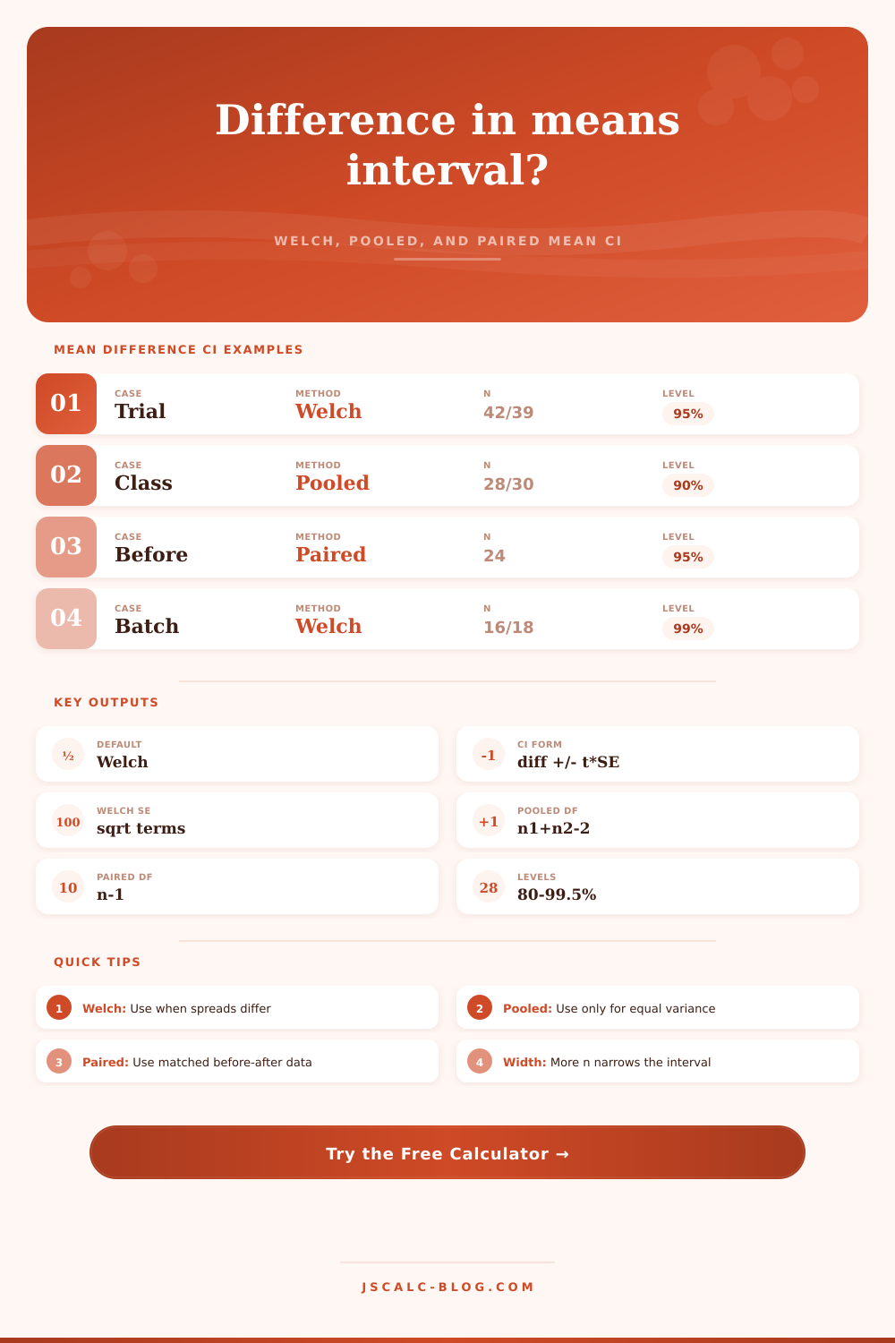
Calculate a two-sided confidence interval for mean1 minus mean2 using Welch's method, a pooled equal-variance method, or a paired mean-difference method.
Load a realistic comparison, then change the sample summaries, confidence level, and method.
Enter summary statistics to calculate a confidence interval.
| Quantity | Symbol | Your value | Role in formula | Method note |
|---|---|---|---|---|
| Enter statistics above to calculate the interval. | ||||
| Method | When to use | SE formula | Degrees of freedom | Variance assumption |
|---|---|---|---|---|
| Welch independent | Two independent groups with possibly unequal SDs | sqrt(s12/n1 + s22/n2) | Welch-Satterthwaite | Unequal variances allowed |
| Pooled independent | Two independent groups with similar spreads by design | sp sqrt(1/n1 + 1/n2) | n1 + n2 - 2 | Equal variances assumed |
| Paired difference | Matched, repeated, before-after, or same-subject data | sd / sqrt(n) | n - 1 | Uses SD of within-pair differences |
| Large sample z check | Rough comparison when df is very high | Same SE as selected t method | Very large df | Critical value approaches z |
| Planning shortcut | Early sample-size sketches | Expected SD times root terms | Expected df | Replace sample SDs after data arrive |
| Confidence level | Tail alpha | Approx z | Effect on CI | Common use |
|---|---|---|---|---|
| 80% | 0.100 each | 1.282 | Narrowest listed interval | Quick exploratory screen |
| 90% | 0.050 each | 1.645 | Moderate interval width | Pilot studies and operations |
| 95% | 0.025 each | 1.960 | Standard reporting level | Most research summaries |
| 98% | 0.010 each | 2.326 | Wider than 95% | Stricter uncertainty reporting |
| 99% | 0.005 each | 2.576 | Wide interval | High-confidence decisions |
| 99.5% | 0.0025 each | 2.807 | Widest listed interval | Very conservative summaries |
| Scenario | Likely method | Inputs to collect | Common df cue | Interpretation focus |
|---|---|---|---|---|
| Randomized two-arm trial | Welch or pooled | n, mean, sample SD by arm | Welch df often fractional | Estimate treatment minus control |
| Two class sections | Pooled if rubrics match | section means, SDs, n | n1 + n2 - 2 | Academic score gap |
| Before-after measurements | Paired | mean and SD of differences | pairs minus 1 | Average within-person change |
| Two production batches | Welch | batch means, SDs, counts | depends on variance terms | Practical process shift |
| A/B test continuous metric | Welch | mean, SD, completed users | large when samples are large | Lift in original metric units |
| Matched instruments | Paired | difference per item | matched pairs minus 1 | Bias between instruments |
So you do a split test on your site: one page has a red button, another page has a green button. Your conversion rate was a bit higher with the green button but is that real? Is that a real win or just noise? That’s where statistics come in to answer the question.
And that’s why you want a confidence interval for the difference in means. The raw difference between two average is called the point estimate, and most folks stop there. They find a three point lift and celebrate. However, that single number hide the uncertainty surrounding the estimate.
What is a Confidence Interval?
A confidence interval wraps all that uncertainty up in a range, providing you with a realistic window into what the true effect is probably like. It turns a guess into a bounded estimate.
Unless you have a compelling reason to think the variance between groups are equal, use the Welch’s method. This option appear to be the one you’ll want most of the time. With two independent groups, there’s no way to know if they match up on their distribution of scores. It could be that Group A has a tighter spread than Group B or vice versa. Welch’s method account for this (by adjusting the degrees of freedom). So even though it’s a tiny technical detail, it ensures you aren’t too confident about your conclusion. That little bit of wiggle room is built into the bounds you’re seeing.
That’s the math. How do you perform it?
Here’s where I plug in the right formula for each of those methods. Enter number of participants per group and select which type of test you’d like to run. The tool calculates everything for you… Giving you the important t value and the standard error. You can see how far off the mark you may be. There ya go!
But with paired data, you need to think about it completely different. Here you are looking at how much things change from before to after measurements on same people. You are not looking at two independent group that each has their own pool of variance. In this case, the calculator flips its inputs because it’s asking for the standard deviation of the differences (not the raw standard deviations for both groups), which makes all the difference in the world.
When you feed it the wrong standard deviation, it increase the error term and thus expands the interval unnecessarily, making it wider then it needs to be. It becomes the difference between measuring the noise in the signal itself vs. Measuring the noise in the players. Once you’ve got the difference scores correct, the interval shrinks and reveal effects you otherwise wouldn’t see with independent methods.
The width of the interval tells a story about your sample size and your chosen confidence level. Why do we use a 95 percent interval as the default? Because it strikes a balance between being certain (but not precisely) right. Crank that number up to 99 percent and what happens? The interval gets wider. You’re asking for more certainty, and that costs you in terms of a less-precise estimate. In exchange for gaining confidence, you lose detail. It’s a tradeoff you has to make explicitly.
Wide intervals from small samples indicate too much room for error. Narrow windows emerge when you have large samples, they tend to squeeze the true effect into a tight range. This is where power becomes important.
When your interval contains zero then you can’t rule out that there may be no difference whatsoever. So what you have here is a statistically unclear result.
Half of the work is knowing which to choose. And half is knowing how to interpret those results within the proper context. Not all statistically significant differences is usefully significant in practice. You could discover that the new process actualy only saves two seconds per unit of production with a confidence interval so narrow as to exclude zero. That’s an effect, and it’s statistically significant… But whether or not it’s worth your while on the bottom line is a matter of judgment, not statistics. The stats tell you precisely; you furnish the judgment.
But all told, these intervals are about humility. It is the humility of knowing your sample is simply one piece of a bigger population. It’s somewhere in there, right? The true effect is somewhere in there, so recognize its bounds. Recognize those bounds and you’re being honest with yourself.
Stop chasing individual numbers and start to think in terms of ranges. Doing that will change what you decide. It will make you less prone to the hype, more tuned into the evidence.
The green button could still win, but now you know precisely how certain you can be that it will. And that certainty is worth more than the color of the click.