Confidence Interval for Variance Calculator

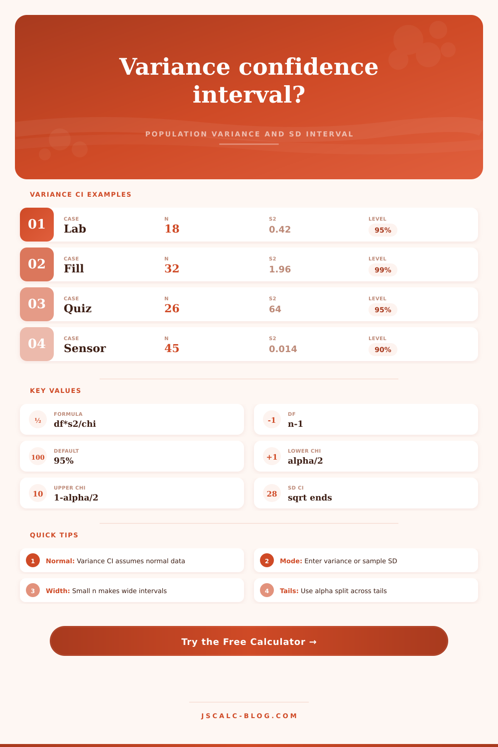
Calculate a confidence interval for a population variance and the matching standard deviation interval using sample size, sample variance or sample SD, degrees of freedom, and chi-square critical values.

📌Presets

Use a real scenario to populate the form, then adjust the sample size, spread measure, and confidence level.

🧮Calculator Inputs

Spread input mode Both modes calculate the same variance interval.

Sample size n Degrees of freedom are df = n - 1.

Sample variance s² Use the sample variance with n - 1 denominator.

Sample standard deviation s The calculator squares this value to get s^2.

Confidence level Alpha is split equally across two tails.

Custom confidence percent Used only when confidence level is Custom.

Measurement units Variance is displayed in squared units.

Reference variance target Optional benchmark for whether a target variance sits inside the CI.

Decimal places Controls interval and critical value rounding.

Critical value method The engine uses inverse chi-square; tables below show common checks.

Normality assumption check The exact chi-square variance CI assumes normal population data.

Show standard deviation interval

Enter n, sample variance or sample SD, and confidence level to calculate the population variance interval.

Variance confidence interval results

Population variance CI -- for σ²

Population SD CI -- square roots of variance endpoints

df and confidence -- alpha split across both tails

Chi-square criticals -- lower quantile / upper quantile

📋Current Interval Grid

17dfn - 1

95%confidencetwo-sided

0.025lower tailalpha / 2

0.975upper tail1 - alpha / 2

s^2input modesample variance

0.420sample variancesquared units

0.648sample SDoriginal units

lookupcritical sourceinverse chi-square

normalassumptionrequired

targetbenchmarkoptional

📚Chi-Square Reference Tables

df	90% CI chi lower	90% CI chi upper	95% CI chi lower	95% CI chi upper	99% CI chi lower
5	1.145	11.070	0.831	12.833	0.412
10	3.940	18.307	3.247	20.483	2.156
15	7.261	24.996	6.262	27.488	4.601
20	10.851	31.410	9.591	34.170	7.434
30	18.493	43.773	16.791	46.979	13.787
50	34.764	67.505	32.357	71.420	27.991

Input mode	Required inputs	Internal variance	Best use	Common mistake
Sample variance s²	n and s²	s²	Statistics software output lists variance.	Using population variance with N denominator.
Sample SD s	n and s	s x s	Reports list standard deviation only.	Forgetting to square s before the variance formula.
Target variance	Optional benchmark	No interval change	Check if a specification variance is plausible.	Treating inside CI as proof of equality.
Custom confidence	50% to 99.9%	Changes alpha	Planning sensitivity or matching a protocol.	Entering 0.95 instead of 95 in percent field.
Normality note	Judgment from data	No interval change	Document whether the exact CI assumption is credible.	Using exact chi-square CI for heavily skewed data.
Decimal places	1 to 5	No interval change	Match lab, quality, or classroom reporting precision.	Rounding criticals before final calculation.

Scenario	Typical n	Common level	Variance question	Interpretation focus
Lab repeatability	10 to 30	95%	How large could method variance be?	Upper bound for quality review.
Manufacturing fill	25 to 60	99%	Is process spread under control?	Variance target inside or outside CI.
Education scores	20 to 80	95%	How uncertain is score variability?	SD interval in original points.
Sensor calibration	30 to 100	90%	Is short-term drift variance stable?	Narrowness from larger df.
Clinical marker	15 to 50	95%	What range of population SD is plausible?	Assumption check before planning.
Delivery operations	40 to 200	90%	How variable are elapsed times?	Skew caution for time data.

Quantity	Formula	Uses df?	Reported by calculator
Degrees of freedom	df = n - 1	Yes	Card and breakdown
Tail alpha	α / 2 and 1 - α / 2	No	Grid and critical lookup
Lower variance bound	df x s² / χ²_1-α/2,df	Yes	Primary CI
Upper variance bound	df x s² / χ²_α/2,df	Yes	Primary CI
Lower SD bound	sqrt(lower variance)	No	Secondary CI
Upper SD bound	sqrt(upper variance)	No	Secondary CI

🔢Formula Breakdown

Variance interval( (n - 1)s² / χ²_upper, (n - 1)s² / χ²_lower )

Critical valuesχ²_lower = χ²_{α/2, df} and χ²_upper = χ²_{1-α/2, df}, with df = n - 1.

SD intervalTake the square root of each variance endpoint to return to the original measurement units.

Lookup / approxThe calculator numerically inverts the chi-square CDF; the Wilson-Hilferty approximation supplies the starting point before bisection refinement.

💡Practical Tips

Assumption tip: The classic chi-square variance interval is exact for normal population data. For skewed measurements, review a plot or use a method matched to the data-generating process.

Interpretation tip: The variance interval is naturally asymmetric. Report the SD interval alongside it when readers need spread in the original units.

In nearly all planning situations there will be variability. With some reasonable ease we may calculate mean or average of whatever it is we are measuring (e.g., average lab result, average delivery time). But where’s the story? That’s usually found in the spread of the numbers. Use the variance confidence interval calculator to measure uncertainty.

Enter your sample data to construct a range on the population variance. Then, convert that endpoint to standard deviation interval. Now you have better picture of what’s going on in your process.

Why You Should Measure Spread, Not Just Average

Why? Because we used the chi-square distribution for the math. The chi-square isn’t symmetric like bell curve. It is a one-sided, skewed distribution that produces an uneven interval. The upper and lower bounds aren’t equidistant from sample variance. That curvature are taken into account with the calculator; they plugs in your sample size (minus 1, because it’s called “degrees of freedom”) and calculate proper critical values. These then divide sample variance in the appropriate way, based off whether you’re in the left or the right end of the distribution.

And it require normal data. To be clear: The base population must be normally distributed. That’s the bit where folks stumble. Skewed data can throw off the interval. For example, delivery times might pile up around zero, with a long tail to the right. Your confidence intervals won’t cover the true variance as frequent as you believe.

That’s why there’s an option in the tool to check if your data is normal. This is a gentle nudge toward inspecting your Q-Q plot (or histogram). Go check. Then believe. Because without the assumption, the interval is misleading and you’re thinking you have control when you’re actualy adrift.

The range will also be a function of sample size. A small number yields a wide range. Makes sense. If you measure just eighteen things, you know less different than if you measure eighty. Degrees of freedom in calculator reflect that. As the sample size grows, the chi-square distribution tightens, which make your interval narrow. Look at the critical values by degrees of freedom in reference table on the page. See how they change? And as the sample increases, they get closer. Which is why quality engineers is such nuts about replication. More data reduces the uncertainty.

Enter sample standard deviation or sample variance. (If you select the latter, the calculator will squares the value of the former.) No statistical change here, but just a convenience feature. Because the standard deviation has the same units as your measurements, many reports provide this number instead. The variance, however, is in squared units and can be hard to grasp. The tool provides both. While the variance interval describes the spread in statistical terms, the standard deviation interval change that to something you can put to use. If your measurements are in milliliters, then you want your interval to be in milliliters, too… Not milliliters squared.

The calculation is less important than the interpretation. The fact that your confidence interval includes some range doesn’t mean that the true variance lies there with certainty. What it means is that when done repeatedly on different samples, the method will captures the truth a given percentage of times. For example, a 95 percent interval means that 95 percent of intervals constructed like that will include parameter. That’s an important and subtle difference. Does this particular interval fall into the set of winners? Or the losers? No idea. But you should of trust the method.

Check benchmarks in the target variance field. In other words, look at the lower and upper bounds of the process variation to see if they falls below the benchmark you entered in the target variance field. Does the top end of your variation exceed the target? Then you know that you don’t have a capable process. Perhaps you do; maybe you just haven’t sampled enough or controlled well enough. The calculator make this obvious. There is no guesswork.

Variance tells a story that averages conceal. Two processes may share the same average yet differ greatly in their spread. One is a gamble. The other is reliable. By quantifying this spread, you can then make decisions that account for risk, not hope. The interval provides a limit on how much the worst case might change. This is information required to set safety stocks, build capacity, or approve a new method. To know where you stand, you measure the center. To know how stable you are, you measure the spread. It’s stability that keeps the lights on.