Correlation Coefficient P Value Calculator
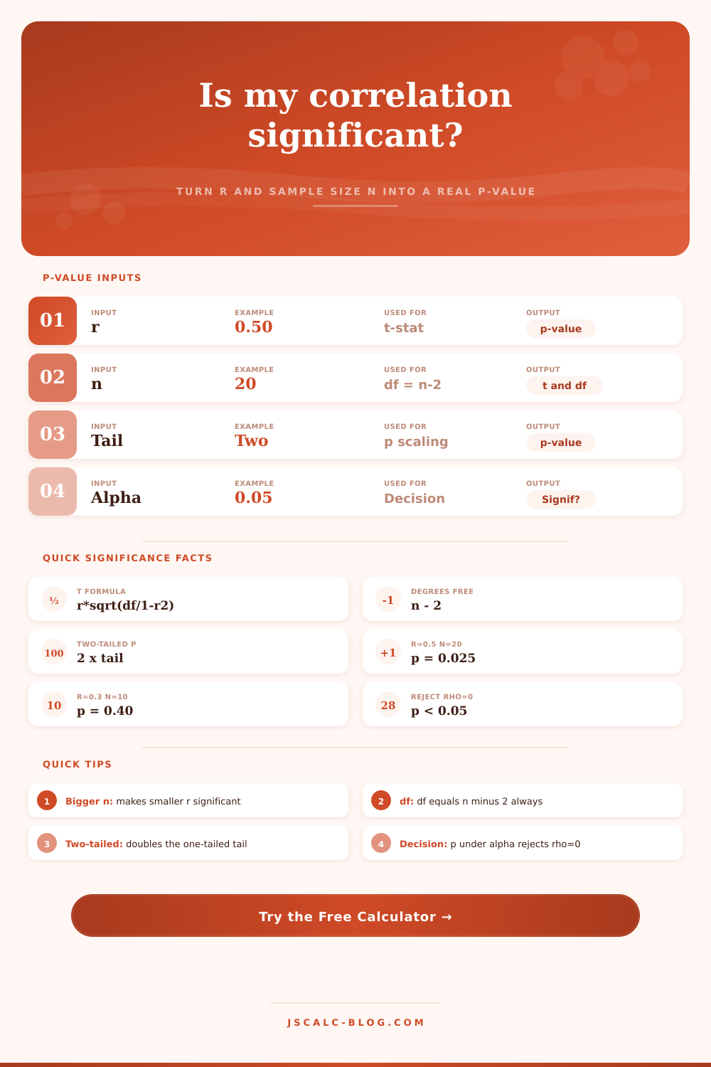
Enter a Pearson correlation r and the sample size n to get the t-statistic, degrees of freedom, and the two-tailed or one-tailed p-value for the hypothesis test that the true correlation ρ equals zero.
🎯Real r and n Presets
📝Test Inputs
Pearson r between the two variables.
Number of paired observations; df = n – 2.
🔢Formula Snapshot
⚙How The P-Value Is Built
📊Critical r by Sample Size (Two-Tailed)
| n (pairs) | df = n – 2 | Critical r at 0.05 | Critical r at 0.01 | Meaning |
|---|---|---|---|---|
| 5 | 3 | 0.878 | 0.959 | Need very strong r |
| 10 | 8 | 0.632 | 0.765 | Strong r required |
| 15 | 13 | 0.514 | 0.641 | Moderate to strong |
| 20 | 18 | 0.444 | 0.561 | Moderate r works |
| 25 | 23 | 0.396 | 0.505 | Moderate r works |
| 30 | 28 | 0.361 | 0.463 | Smaller r counts |
| 50 | 48 | 0.279 | 0.361 | Weak r can pass |
| 100 | 98 | 0.197 | 0.256 | Very weak r passes |
| 200 | 198 | 0.139 | 0.182 | Tiny r significant |
📉Critical t by Degrees of Freedom
| df | t at 0.10 | t at 0.05 | t at 0.01 | t at 0.001 |
|---|---|---|---|---|
| 3 | 2.353 | 3.182 | 5.841 | 12.924 |
| 6 | 1.943 | 2.447 | 3.707 | 5.959 |
| 8 | 1.860 | 2.306 | 3.355 | 5.041 |
| 13 | 1.771 | 2.160 | 3.012 | 4.221 |
| 18 | 1.734 | 2.101 | 2.878 | 3.922 |
| 23 | 1.714 | 2.069 | 2.807 | 3.768 |
| 28 | 1.701 | 2.048 | 2.763 | 3.674 |
| 60 | 1.671 | 2.000 | 2.660 | 3.460 |
| 198 | 1.653 | 1.972 | 2.601 | 3.340 |
Two-tailed critical values. One-tailed tests use the alpha column for the matching one-sided level.
🗂Comparison Grid: r and n vs t, df, p
| r | n | df | t-statistic | Two-tailed p | Significant at 0.05 |
|---|---|---|---|---|---|
| 0.50 | 20 | 18 | 2.449 | 0.0248 | Yes |
| 0.80 | 15 | 13 | 4.807 | 0.0003 | Yes |
| 0.20 | 30 | 28 | 1.080 | 0.2893 | No |
| 0.30 | 10 | 8 | 0.889 | 0.3997 | No |
| 0.10 | 200 | 198 | 1.414 | 0.1589 | No |
| 0.95 | 8 | 6 | 7.452 | 0.0003 | Yes |
| 0.45 | 25 | 23 | 2.417 | 0.0240 | Yes |
| -0.60 | 18 | 16 | -3.000 | 0.0085 | Yes |
| 0.36 | 30 | 28 | 2.043 | 0.0505 | No (just over) |
| 0.70 | 5 | 3 | 1.699 | 0.1878 | No |
📋P-Value and Effect Size Guide
| Range | P-Value Reading | |r| Effect Size | Practical Meaning |
|---|---|---|---|
| p < 0.001 | Very strong evidence | 0.50 to 1.00 | Large correlation |
| 0.001 to 0.01 | Strong evidence | 0.30 to 0.50 | Moderate correlation |
| 0.01 to 0.05 | Moderate evidence | 0.10 to 0.30 | Small correlation |
| 0.05 to 0.10 | Weak or borderline | 0.05 to 0.10 | Very small effect |
| p ≥ 0.10 | Little evidence | 0.00 to 0.05 | Negligible effect |
Effect-size bands follow Cohen. A small p can pair with a small r when n is large, so report both.
💡Reading The Result
Take your correlation coefficient, which shows a correlation of 0.5 between two variables. That’s pretty impressive, unless you consider it came from a mere sample size of ten. With such a small group, even moderate relationship appears as just noise pretending to be signal.
Here’s where statistical significance comes in: Does the observed relationship have a plausible probability of occurring at random? The purpose of this calculator is to answer that question. Feed it your Pearson r, along with your sample size n, and it will spit out a p-value, degrees of freedom, and t-statistic, all useful for assessing whether your observed relationship is likely to be real or if there is a reasonable likelihood that the true correlation in the population are zero (i.e., the null hypothesis).
How to Use This Calculator
But take away the jargon, and it’s pretty simple. Give it two values, the number of observations you’ve paired together, and the strength of their connection (the correlation). And let the machine do its thing.
How does it work? First, it determines the degrees of freedom. Here’s how many: Take your sample size and subtract two. Why? Because when you estimate the correlation, you’re using up two degrees of freedom within your dataset. Next, it takes r and converts it into a t-statistic. In other words, it uses an equation that considers the strength of the relationship AND how much uncertainty still remains in your dataset. That’s the math that provides the connection between our t-statistic and a table of standard distributions, which we can use to determine statistical significance.
In statistics, sample size is the great equalizer. With enough data points, even a tiny correlation is highly significant. But with too few observation, even a massive correlation fails to reach significance. Thankfully, the calculator handles those trade-offs on your behalf. There’s no more manually looking up tables or fiddling with complex spreadsheet formulas.
Simply choose between a one-tailed and a two-tailed test. Two-tailed tests check both positive and negative deviations from zero, this is the safer default for most exploratory research. One-tailed tests assume a direction ahead of time; it doubles your statistical power but also requires stronger justification.
But what does p mean? To understand the output, we need to know what p actualy means. It’s not the probability that your hypothesis is true. Rather, it’s the probability of seeing such an outcome in your data if there was really no relationship in the population. If p is lower than your selected alpha threshold (typically 0.05), then you’ll reject the null hypothesis. You’ll conclude that the correlation are statistically significant.
But here is where many researchers fall into a trap: just because something is statistically significant doesn’t mean it’s important. With a large enough sample size, even a trivial correlation can be made statistically significant. Researchers ends up overconfident about a weak relationship. Numbers without context are meaningless.
Take this example: A researcher discovers a high positive correlation between shark attack and ice cream sales, which holds up to all statistical significance tests. This means you have found a very unlikely pattern to occur through random chance. Does this mean eating ice cream makes you more likely to get attacked by sharks? No one with any common sense will tell you so. There’s a third factor at play here: Summer heat! The statistical test doesn’t prove causation, it simply indicates that there’s an unlikely-to-be-random-pattern. It can’t discount possible confounders either. That part of interpretation requires you to know something about the problem domain yourself.
The tool also includes a few other highlights, such as handy reference tables that show which correlations is significant at different sample sizes. For instance, if you have just 20 pairs, then your correlation needs to be about 0.44 to jump over the 0.05 hurdle. If you have two hundred pairs? You can squeak past with a correlation as low as 0.14. This underscores how much easier it is to identify smaller effects with bigger samples, and why replication matters so much in science. A seeming groundbreaking result in a small pilot study may simply dissapears with a bigger-scale test with more rigorous criteria.
The complete story requires reporting both the p-value AND the effect size. How strong’s the link? This is the correlation coefficient. Can I believe in the existence of this link or not? Combined, they protect against misunderstanding. You get a significant result, great! But the r value barely exceeds 0. What good is it? It’s statistically real but perhaps practically useless.
Then there is the large r paired with a borderline p-value. It would of been time to collect some more data instead of throwing up our hands.
The bottom line: The test’s not the point. To me, understanding something about how things relate in the real world is the point. Judgment gives numbers their meaning; the structure comes from the numbers. Whether you’re looking at the results of an experiment, a survey, or observational records, keep in mind that significant just begins the conversation. Yes, it tells you the pattern exists. Now go work to determine what it realy means. And that’s where the difference between being a good analyst and a wise one lies. It converts raw output into useful information you can use.