Confusion Matrix Calculator
Enter true positives, false positives, false negatives, and true negatives to calculate accuracy, precision, recall, specificity, F1 score, MCC, and classification error patterns from one 2x2 matrix.
🎯Confusion Matrix Presets
📝Classification Inputs
Sets the wording used in the interpretation notes.
Name the target class, disease, defect, alert, or event.
Name the non-target class or normal condition.
Predicted positive and actually positive.
Predicted positive but actually negative.
Predicted negative but actually positive.
Predicted negative and actually negative.
Controls percentages and decimal metrics.
🧮Metric Summary Grid
📋Current Confusion Matrix
📐Metric Formula Table
🔎Preset Comparison Table
| Preset | TP | FP | FN | TN | Best metric to watch |
|---|---|---|---|---|---|
| Rare fraud alerts | 145 | 310 | 55 | 99490 | Precision and MCC reveal false-alert load. |
| Spam filter batch | 8420 | 610 | 880 | 20090 | F1 balances blocked spam and missed spam. |
| Cancer screening audit | 92 | 45 | 8 | 855 | Recall matters when misses carry high risk. |
| Vision defect line | 318 | 132 | 42 | 9508 | Specificity controls rework volume. |
| Churn risk model | 620 | 780 | 340 | 3260 | Precision tells how focused the outreach list is. |
| Search relevance classifier | 2210 | 390 | 290 | 4110 | Accuracy and F1 both stay useful. |
| Loan default monitor | 430 | 920 | 170 | 8480 | MCC resists the class imbalance. |
| Wildlife camera detector | 760 | 180 | 240 | 3820 | Recall and false negatives guide tuning. |
| Emergency triage model | 146 | 160 | 4 | 690 | Recall dominates for rule-out safety. |
| Quality retest gate | 64 | 80 | 16 | 1840 | Low prevalence makes PPV sensitive to FP. |
⚖Interpretation Bands
| Metric | Lower range | Middle range | Higher range | What it controls | Caution |
|---|---|---|---|---|---|
| Accuracy | Below 70% | 70% to 90% | 90%+ | Overall correct share | Can look high with rare positives. |
| Precision | Below 50% | 50% to 80% | 80%+ | Quality of positive predictions | Ignores false negatives. |
| Recall | Below 50% | 50% to 80% | 80%+ | Capture of actual positives | Ignores false alarms. |
| Specificity | Below 70% | 70% to 95% | 95%+ | Clearance of actual negatives | Does not show missed positives. |
| F1 score | Below 50% | 50% to 80% | 80%+ | Precision-recall balance | Does not use true negatives. |
| MCC | Below 0.20 | 0.20 to 0.60 | 0.60+ | All four matrix cells | Undefined when a marginal is zero. |
💡Confusion Matrix Tips
This calculator uses the standard binary-classification formulas from the four raw cells TP, FP, FN, and TN. Validate threshold choice, sample design, and labeling quality before using the metrics for operational decisions.
Is this a fraud? Will I get cancer from this tumor? Is this email spam? It sounds like a simple yes/no question, but the answer never come so easily.
Maybe we’ll run a prediction model to determine whether a transaction is fraudulent. Or maybe a diagnostic test will indicate that there’s something amiss. Or perhaps our spam filter flags a phishing link. At first glance, it appear that we’ve got the problem solved.
Why Accuracy Is Not Enough
But there is a dirty little secret in data science: the right prediction isn’t worth anything unless we understand how much it costs to be wrong. So instead of simply looking at headline accuracy score, we look deeper into confusion matrix. And that’s where the calculator above comes in, converting raw numbers into easy-to-understand performance metrics. But knowing what they mean doesn’t come from plugging them in; you have to know what they represent.
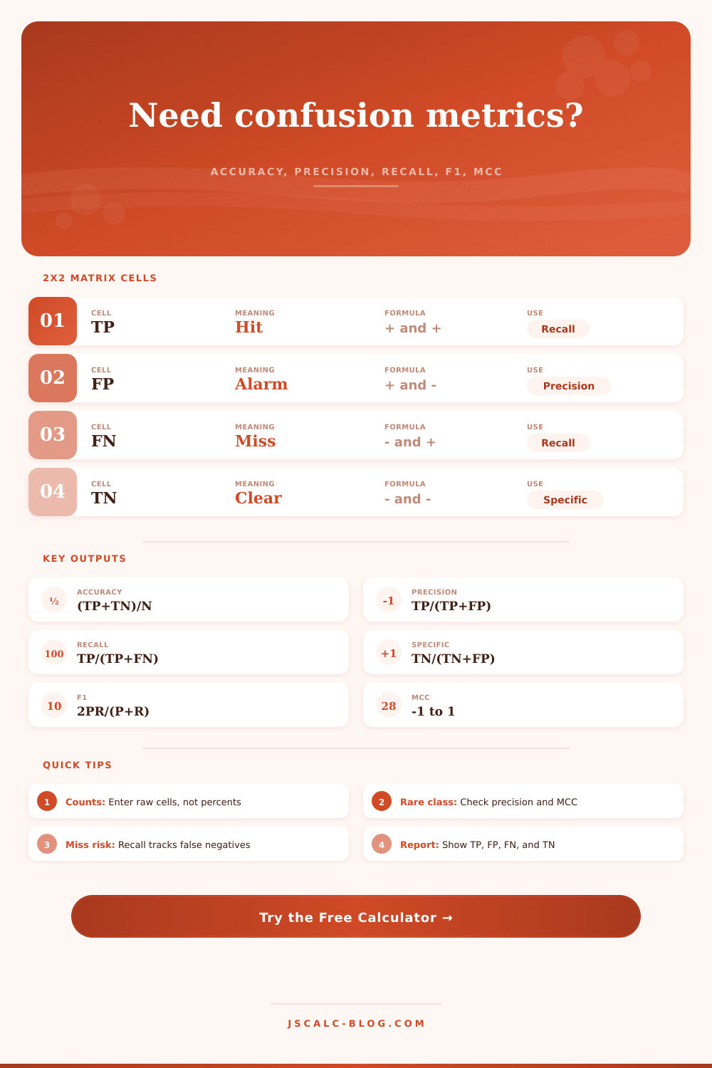
This brings us back to our 2×2 table of true positives/false positives/false negatives/true negatives. This is the basic table that everything else is built on. It’s what your classifier does, four cells, each with its own story to tell.
Your hits are the true positives. And your quiet moments, when it got it right and didn’t bother, are the true negatives.
Then there are the errors. Your false positives are the alarms that proved to be nothing, wasting resources and time. And your false negatives are the silent failures, the threats or diseases that slipped through the net.
That’s the central tension in every binary classification problem: You can’t eliminate both errors at once, unless you also improve the signal underneath. So you must decide how much of either one you can live with less then the other.
People make this mistake: they consider overall accuracy and assume that they’re fine. Then they realize their model never works. A model that just returns ‘healthy’ all the time will be 99.9% accurate. Sounds great! But what if you’re screening for a rare disease with one-in-a-thousand rate? This model won’t find any patient. Accuracy is seductive because it’s simple to grasp, but it can be blind to class imbalance.
Also, precision and recall matter. Precision protects you from false alarms: how many of your positive predictions were actualy correct? Recall protects you from misses: how many of the actual positives did you manage to catch? You can think about this tension as trade-offs.
The calculator reminds you of them and even gives you an overall score that balances those competing needs, which is the F1 score (also known as the harmonic mean of recall and precision). That means you have to admit that raising your score on one will tend to lower it on another. For example, if you make your positive prediction threshold more lenient, you will increase your recall… You’ll catch more true positives; but you’ll also pick up more false positives, lowering your precision.
The F1 score penalizes dramatic differences between the two, so you get a single number that captures how well model does at both. That’s a nice summary, though it has one major blind spot: it doesn’t consider true negatives at all, which can be a big problem in certain contexts.
The Matthews Correlation Coefficient (MCC) is where it’s at. Unlike the F1 score, the MCC considers all four cells in your confusion matrix. It’s a solid metric. Even if your data is highly imbalanced, it will give you a high score as long as you’re doing well on both classes. In other words, it’s robust and only gives you a high score when you’ve gotten good results across both classes. If it predicts perfectly, you’ll get a score of 1; if it predicts randomly, you’ll get a 0; if it completely disagrees with what you want, then -1. Basically, MCC is mathematically stricter and tends to be more honest about how well you’re performing compared to accuracy or F1. See here for a clear reference table that explains how each metric reacts to various kinds of errors.
The cost of an error matters in real-world decisions. You can’t miss a case of cancer; tune for high recall (with higher false positives to get tested). You don’t want to miss a legitimate invoice from your supplier; tune for high precision (accepting some spam instead). You need to specify that cost… There’s no single best score here, just the correct one given your own risk tolerance. That’s what this tool helps you quantify.
In the end, that’s what a confusion matrix does: reflect your model’s bias back at you. It tells you who (or what) will pay the price for its mistakes. If you’re screening out patients, fighting spam, or detecting fraud, whatever it is… Then you need to make sure your metrics line up with your values.
Catching the right things doesn’t matter much unless they’re the ones you care about most. What should you catch? What can you miss? That’s on you. The math just makes it clear.