Conditional Probability Calculator
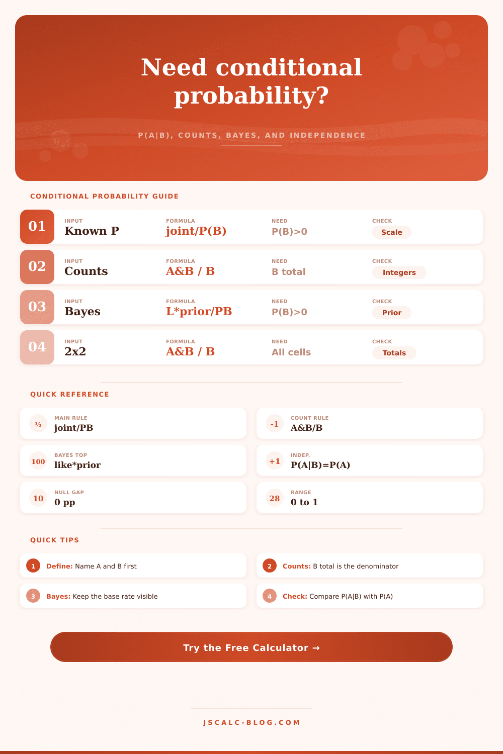
Calculate P(A|B) from known probabilities, counts, 2 x 2 tables, or Bayes inputs, then compare the result with P(A) for an independence check.
🎯Scenario Presets
⚙Conditional Probability Inputs
Choose the data format you have. Each mode returns P(A|B).
The profile changes the wording, not the arithmetic.
All probability fields use the selected scale.
Use more places for small base rates and rare outcomes.
A is the event you want after learning B happened.
B is the condition, filter, test result, or subgroup.
Leave at 0 only when no baseline P(A) is available.
P(B) must be greater than 0.
The joint cannot exceed P(A) or P(B).
Used only for the reverse conditional snapshot.
This is the numerator in count mode.
This is the denominator: P(A|B) = A and B / B total.
Needed to compare P(A|B) with P(A).
Needed to convert the counts into overall probabilities.
Top-left cell: A happens and B happens.
A happens outside the condition B.
This combines with A and B to form the B total.
Completes the 2 x 2 table and all marginal totals.
The base probability before observing B.
How often B appears when A is true.
Overall probability of seeing B.
Displayed as a complement check when it is available.
Base rate of A before the positive signal B.
Positive signal rate among true A cases.
Positive signal rate when A is not true.
Used to show expected counts for the Bayes breakdown.
🔢Current Probability Grid
📋Computed Probability Table
📐Formula Reference Table
| Situation | Use This Formula | Inputs Needed | Output | Watch For |
|---|---|---|---|---|
| Standard conditional probability | P(A|B) = P(A and B) / P(B) | Joint probability and P(B) | Probability of A after B is known | P(B) must be greater than 0 |
| Count mode | P(A|B) = A and B count / B total | Matching count and denominator count | Observed conditional rate | Use counts, not row percentages |
| Bayes relation | P(A|B) = P(B|A) x P(A) / P(B) | Prior, likelihood, and evidence | Posterior probability | Base rate strongly affects the result |
| 2 x 2 table | P(A|B) = cell A and B / column or condition B total | Four cell counts | Conditional rate plus margins | Confirm which event is A and which is B |
| Independence check | Compare P(A|B) with P(A) | Conditional rate and baseline P(A) | Difference in percentage points | Equality suggests independence in that direction |
| Reverse conditional | P(B|A) = P(A and B) / P(A) | Joint probability and P(A) | Probability of B after A is known | Do not swap it with P(A|B) |
🧭Preset Comparison Table
| Preset | Mode | Event A | Condition B | Typical P(A|B) | Main Lesson |
|---|---|---|---|---|---|
| Rare disease screen | Diagnostic Bayes | Condition present | Positive test | 15% to 20% | Good sensitivity can still leave modest posterior probability when the base rate is low |
| Fraud alert review | Diagnostic Bayes | Fraudulent transaction | Model alert | 10% to 15% | False positives dominate when true fraud is rare |
| Email click given open | Count mode | Clicked | Opened email | 13% to 14% | The denominator is open count, not total recipients |
| Night shift defect | 2 x 2 counts | Defect | Night shift | 4% to 5% | Compare with overall defect rate before calling the shift unusual |
| Pass given attendance | Count mode | Passed final | High attendance | 86% | Conditional rate can be much higher than the baseline |
| Delay given heavy rain | Known probabilities | Train delay | Heavy rain | 40% | Joint probability divided by P(B) isolates the rainy subset |
| Escalation given enterprise | 2 x 2 counts | Escalated ticket | Enterprise customer | 16% | A subgroup can have a higher conditional support rate |
| Defect given flag | Bayes relation | True defect | Inspection flag | 15% to 16% | Bayes combines prior defect rate with the flag likelihood |
| Renewal given app use | Known probabilities | Renewed | Used mobile app | 75% | Conditional rates can summarize segment behavior |
| Independent button check | Known probabilities | Converted | Saw blue button | 14% | Matching P(A|B) and P(A) is an independence signal |
🔍Interpretation Checks Table
| Diagnostic | Value to Compare | Near-Zero Cue | High Cue | Plain Reading |
|---|---|---|---|---|
| Independence gap | P(A|B) - P(A) | Within +/- 1 pp | 10+ pp | B changes the observed probability of A when the gap is not near zero |
| Conditional lift | P(A|B) / P(A) | 0.95 to 1.05 | 2.00+ | A lift above 1 means A is more common inside B than overall |
| Denominator health | P(B) or B total | Very small | Stable count | Small denominators make the conditional probability jumpy |
| Joint plausibility | P(A and B) | Not above either event | Close to P(B) | If joint equals P(B), nearly every B case is also A |
| Reverse conditional | P(B|A) | May differ a lot | Often useful | P(A|B) and P(B|A) answer different questions |
| Bayes evidence | P(B) | Derived from all ways B occurs | Clear base rate | Evidence is the normalizing denominator in Bayes calculations |
💡Conditional Probability Tips
Does one event cause another? Or is this a coincidence?
For example, suppose it’s raining as you wait for your train. Trains can be late, and it might be because rain makes tracks slippery. But do you know whether the rain itself caused the train to be late?
Why Conditional Probability Matters
Basic probability give you the frequency of “it rained” or the frequency of “the train was late.” Conditional probability gives you the frequency of “the train was late given it rained.” This make a huge difference in how you think about problem.
Everyone knows simple probabilities: draw a marble out of a bag. In real life, however, one event usually impacts likelihood of another. You might be told event B occurred and this change the probability picture. The calculator perform the necessary math. It divides the joint probability of both events by the probability of the condition to isolate the subgroup in which you’re interested. No need for you to guess at conversions or coefficients.
But it’s all about knowing what to measure. When you’re in count mode, for example, you enter the number of times both A and B happened, and total number of times B happened. And here’s where the denominator matter.
If you’re looking at email marketing, for instance, A could be “clicked the link,” and B could be “opened the email.” You want clicks divided by openers, not divided by total number of recipients. What happens after someone opens a mail doesn’t matter if they didn’t even open it. A lot of people use incorrect denominator, so they dilut the signal.
But Bayes’ theorem make things more complicated by reversing the event relationship. Usually we’re aware of the likelihood of getting a certain test result when you have a condition. But what we’d like to know is probability of having the condition if we get a certain result from the test. Enter the calculator: plug in the evidence, likelihood, and prior probability. This is key for medical screening. Even with an accurate test for a rare disease, a positive result could still indicate that you probably don’t have the disease. The base rate anchors the final probability. Without this anchor, we risk mistaking a positive test as a definite diagnosis.
Finally, it’s good for testing independence. Are the events independent? In other words: Does knowing that B occurred affect the chances of A? The calculator displays this gap right there. A narrow gap indicates that B doesn’t move A’s odds much one way or another. A wide gap tell us that B is a strong indicator of something. So now you have an idea about whether two variables are connected, or merely floating close together by coincidence.
The world doesn’t work in clean datasets. You’ll see tiny denominators with small sample size. Then that one data point has enough power to move the percentages around like crazy. That’s why the reference table says, look at what you put into this equation. If your denominator is really small, then the conditional probability is shaky. It’s just noise. You should of trust it when you have a stable denominator.
Conditionals make you think precisely. They force you to clarify what’s being asked. Are you interested in a certain population? Or are you interested in a sub-population within that larger group? That’s easy math, provided you’re careful with the setup. What are the events we want to describe? Label them. Call them A and B. Count them appropriately. Apply division. And poof! Feeling becomes proof. Now you realy can know whether the train was delayed because it rained.