Bayes Theorem Calculator
Update P(A) after evidence B using the standard Bayes formula, compare likelihood ratios, false positives, diagnostic PPV-style inputs, odds form, and sensitivity across base rates.
🎯Bayes Scenario Presets
📝Bayes Inputs
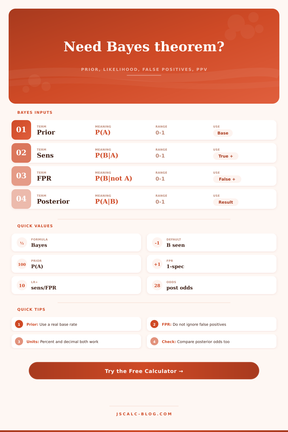
Base rate before seeing evidence B.
Diagnostic equivalent: sensitivity or true-positive rate.
Diagnostic equivalent: 1 minus specificity.
🔢Bayes Symbol Snapshot
📐Bayes Formula Reference
| Quantity | Formula | Meaning | Diagnostic name | Watch for |
|---|---|---|---|---|
| Prior | P(A) | Chance before evidence | Prevalence | Base-rate error |
| Complement | P(not A) = 1 – P(A) | Chance A is false | No condition | Must match prior |
| Likelihood | P(B|A) | Evidence rate when A is true | Sensitivity | Low values miss cases |
| False positive | P(B|not A) | Evidence rate when A is false | 1 – specificity | Can dominate rare priors |
| Evidence rate | P(B|A)P(A)+P(B|not A)P(not A) | Overall chance of B | Positive-test rate | Denominator of Bayes |
| Posterior | P(A|B) = numerator / denominator | Updated chance after B | PPV | Not the same as sensitivity |
🔍Diagnostic PPV Style Examples
| Scenario | Prior | Sensitivity | False positive | Posterior if positive | Why it matters |
|---|---|---|---|---|---|
| Rare screen | 1% | 95% | 5% | 16.1% | False positives outnumber true positives |
| Moderate clinic | 10% | 92% | 8% | 56.1% | Prior makes the same test more persuasive |
| High-risk group | 40% | 90% | 10% | 85.7% | Base rate and evidence reinforce each other |
| Quality sensor | 3% | 88% | 4% | 40.5% | Inspection flags still need confirmation |
| Spam classifier | 30% | 94% | 7% | 85.2% | High prior improves trust in the flag |
| Fraud alert | 0.8% | 85% | 1.5% | 31.3% | Very low prior keeps posterior moderate |
| Weather radar | 25% | 80% | 15% | 64.0% | Evidence shifts the forecast but not to certain |
| Negative result | 10% | 95% | 5% | 0.6% | Absent evidence can strongly reduce probability |
📊Current Sensitivity Grid
⚖Likelihood Ratio Lookup
| LR band | Positive evidence strength | Example input pair | Posterior effect | Common caution |
|---|---|---|---|---|
| 1.0 | No update | 80% / 80% | Prior unchanged | Evidence is not diagnostic |
| 1.5 to 2 | Small lift | 60% / 35% | Gentle movement | Base rate still dominates |
| 2 to 5 | Useful lift | 80% / 25% | Clear but not final | Confirm if decision is costly |
| 5 to 10 | Strong lift | 90% / 12% | Large posterior jump | Input accuracy matters |
| 10 to 20 | Very strong lift | 95% / 6% | Often decisive | Rare priors can still surprise |
| 20+ | Extreme lift | 98% / 2% | Posterior can approach 1 | Validate independence and sampling |
⚙Full Formula Breakdown
💡Bayes Calculation Tips
Screening tests can cause your heart to skip a beat: you get the results and they are positive! The test say you have the condition, but then the doctor hesitates to tell you. Why? More often than not it’s not because the machine is busted. It’s because the machine doesn’t understand the neighborhood or how common this condition is where you live.
Bayes theorem is the mathematical tool that plugs that hole and lets you revise your beliefs as new evidence pours in. Most of us intuitively believe that if test is very accurate, a positive result must be close to certainly true. That intuition is almost always wrong if the condition we’re testing for are rare.
Why a Positive Test Might Still Be Wrong
It does all of this complicated math for you on calculator up top, and then lets you think about what it all means for your decision. First, enter your base rate (otherwise known as starting chance). That’s the one-in-a-thousand chance that a disease would affect you if you didn’t take the test. That’s the chance you started with. It doesn’t go away just because you took the test even though many people will screw this part up.
Enter in sensitivity and false-positive rate next. The sensitivity represent the percent of the time that the test identifies someone who has disease (if they really do). The false positive rate represent the percent of the time that the test falsely reports that you have the disease when you don’t.
And that’s where the counterintuitive bit come in. If the condition is rare enough, even most accurate test, at 99 percent, can mostly be wrong. Let’s say it has a one percent false positive rate. If only zero point one percent of population has the disease, the sick minority will produce fewer true positives than the healthy majority will false ones.
The calculator illustrates this by showing the posterior probability, your updated chance of having the condition given that you saw that result. And it frequently appears to be far less different than what you thought it would be. That is the whole point. The test merely nudges the probability around the base rate, and truth is anchored by the base rate.
Imagine it’s similar to looking for a needle in a haystack, except most of the hay are shaped like needles and sticks to the needle-shaped things. So you use the test which pulls lots of twigs (that look like needles) along with actual needle. But the more twigs to needles, the less certain you feel about the grab. The ability to switch views to see what’s actualy present/absent in the sample is key.
A negative reading are equally meaningful. If the test can rules things out, a negative result will take your suspicion from ten percent down to almost none. And this is where likelihood ratio becomes so helpful. It gives you a sense of how much stronger or weaker the evidence is by showing how likely you were to see that particular result if you had the condition compared to if you did not. Not? High = strong. Low = weak.
This is logic that doctors apply daily, but they don’t usually bother writing down the equations. They estimate base rate of the disease, then factor in accuracy of their tests. The calculator lets you play doctor, if only temporarily. You force yourself to face the base rate. You let yourself admit that most people don’t have whatever it is your shiny new test pick up.
The reference table on the page spells it out plainly: how different priors will swing the final result wildly. One test could of been incredibly helpful at picking up a problem in high-risk group, while being almost useless as a screener among general public.
And that’s the point: Evidence isn’t absolutes. Evidence is relative to your pre-existing beliefs. Evidence is clues, not verdicts. Running the numbers helps you distinguish between signal and noise. And when you run the numbers, you stop reacting to the headline result; you begin to understand the underlying probability.
This is a small thing. But it makes a big difference. If there’s a 50% chance this will happen, it’ll make me do one thing. If there’s a 99% chance it will happen, it’ll make me do another thing altogether.
Bayes theorem doesn’t simply spit out a number for you. It spits out perspective. You began with a guess. You added some evidence. Now you’ve got a better guess. And that’s the whole point about learning.