Chi-Square Goodness of Fit Calculator
Test whether observed category counts match a hypothesized distribution. Enter counts and expected proportions, then review expected counts, chi-square contributions, degrees of freedom, and the right-tail p-value from the chi-square CDF.
🎯Goodness-of-Fit Presets
📝Test Inputs
Comma-separated labels. The calculator matches labels, observed counts, and hypothesized values by position.
Use frequencies only. Commas, tabs, spaces, or line breaks are accepted.
Enter proportions, percentages, ratios, or expected counts; values are normalized to proportions.
Use 0 for a fully specified distribution; subtract fitted parameters from df.
🔢Current Test Snapshot
📊Observed vs Expected Breakdown
| Category | Observed | Hypothesized p | Expected | O - E | (O - E)^2 / E | Share of X2 |
|---|---|---|---|---|---|---|
| Results load when the calculator runs. | ||||||
🗂Goodness-of-Fit Method Comparison
| Method | Input data | Expected basis | Degrees of freedom | Best use | Main caution |
|---|---|---|---|---|---|
| Pearson chi-square GOF | Category counts | n times hypothesized p | k - 1 - m | Testing a known category distribution | Expected counts should not be too small |
| Uniform GOF | Category counts | Equal proportions | k - 1 | Dice, days, bins, or equally likely choices | Independence of observations still matters |
| Multinomial GOF | One outcome per trial | Specified category probabilities | k - 1 - m | Survey choices or product mix audits | Approximation improves as n grows |
| Distribution fit with fitted parameters | Binned sample data | Fitted model bin probabilities | k - 1 - fitted m | Normal, Poisson, or other model checks | Subtract every estimated model parameter |
| Exact multinomial test | Small category counts | Specified probabilities | Not chi-square df based | Very small samples with sparse expected cells | More computationally intensive |
| Chi-square independence | Two-way count table | Row total times column total / n | (r - 1)(c - 1) | Association between two categorical variables | Different question than one-sample GOF |
📋Degrees of Freedom Examples
| Scenario | Categories k | Estimated parameters m | df formula | df | Why |
|---|---|---|---|---|---|
| Fair six-sided die | 6 | 0 | 6 - 1 - 0 | 5 | All six probabilities are specified as equal |
| Four answer choices, known split | 4 | 0 | 4 - 1 - 0 | 3 | No probability is fitted from the data |
| Poisson count bins, lambda fitted | 6 | 1 | 6 - 1 - 1 | 4 | The rate parameter consumes one df |
| Normal bins, mean and SD fitted | 8 | 2 | 8 - 1 - 2 | 5 | Two model parameters are estimated |
| Too many fitted parameters | 4 | 3 | 4 - 1 - 3 | 0 | The chi-square p-value is not defined |
📑Expected Count and Evidence Checks
| Check | Typical guideline | Pass signal | Warning signal | Action |
|---|---|---|---|---|
| Expected cell size | Every expected count at least 5 | Approximation usually usable | Any E below 5 | Combine defensible categories or use exact methods |
| Total sample size | Larger n improves approximation | Stable expected counts | Very small n | Treat p-value as rough |
| Independence | Each observation belongs to one category | One count per item or person | Repeated or paired counts | Use a model for dependent data |
| Hypothesis specified first | Expected proportions are not tuned after seeing O | Predefined proportions | Post-hoc targets | Report how the target distribution was chosen |
| Significance level | Alpha chosen before testing | p <= alpha rejects fit | Changing alpha after result | Keep alpha fixed in the report |
⚙Formula Breakdown
💡Practical Goodness-of-Fit Tips
When we ask if our observations align with expectations, we are performing a chi-square goodness of fit test. For example, imagine you think a mixed color bag of candy is imbalanced with flavor. Without this tool, you are left with hunches. With it, you go from thinking something smells fishy, to having proof that’s fishy. By running your actual results against your expectations, the test provides statistical support that takes you from suspicious to confident.
No table-hunting required. No complicated formula to memorize. Just use the calculator at the top. Plug in your numbers and hypotheses. Get a decision. This is easy to understand at an intuitive level.
How to Use the Chi-Square Goodness of Fit Test
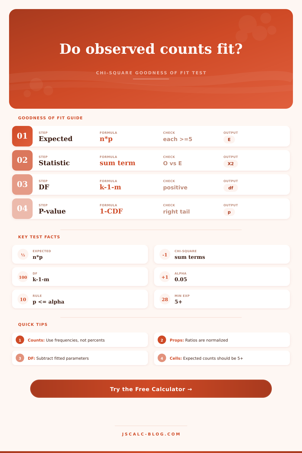
First, come up with some guess or idea as to what distribution of data will look like. Next, gather actual counts from reality and compare them to your hypothesized distribution. The test measures how much they differ. If the two are similar, then it’s reasonable to assume the data conforms to the model. If not, then it doesn’t. How do you decide when a difference is actualy significant? That is measured by how much variation we allow in any given category. One simple measure of this is called the chi-square statistic, a number that sums up overall degree of variance over all categories combined.
But you must discipline yourself to fill in the numbers. Fill in the actual count of how many items falls into each category. That’s the raw frequency, what you saw when you audited or conducted your experiment. Next, fill in the proposed probabilities. Here, again, you have options. You can fill in either exact counts or ratios or percentages of what you expect to see. The software will adjust it for you so that all those proportions add up to 100 percent. Nice, because real world hypotheses aren’t usually nice clean decimals. Maybe you think that two out of every three lights should be red? You type 2 and 1. No need to do the math to get to 0.666 and 0.333. The software fills in the gaps.
The second key parameter is number of parameters we estimate from the data. In the case of testing a die to see if it’s fair, you already have prior knowledge about the probability for every face. So you’re estimating zero parameters. But when you’re testing to see if a dataset fits a normal distribution, you often use the same set of data to find the mean and standard deviation. Each estimated parameter uses up one of the degrees of freedom. Remove that from the category count, and the test becomes more sensitive. The risk you’ll falsely accept a bad fit is lowered.
But the result isn’t just a yes/no answer. Instead, it returns a p-value: how likely you are to see this much difference if your assumption about reality (the hypothesis) is true. If the p-value is low (often considered < 0.05), it means that your observation is unlikely to occur if the model holds. Therefore, you reject the null hypothesis.
That said, the p-value by itself can be misleading. It doesn’t show you specifically what’s causing you to reject the hypothesis. You want to look at the contribution of each category. Many might have contributed substantialy to the overall statistic. These should stand out and help you understand why things don’t fit the model. Is there one particular kind of defect that’s being over-represented? Is there one option on the survey that is completely skipped?
Of course, it has its limitations. You need enough counts per category for the chi-square approximation to work well. For a given cell, that means the expected count needs to be at least 5, based off your sample size. That’s where the assumption about sufficient sample sizes fails. When the expected values fall too low (below 5), then result may not be trustworthy. In those cases, you should of use exact tests and combine sparse categories. The tool warns when such circumstances arises. And it lets you know when you’re trying to make conclusions from wobbly ground.
Another important caveat is the independence of observations. Every data point should be in exactly one category. Observations shouldn’t impact others selection.
This test takes the expectation and pits it against reality. It makes you say up front what you expect will happen before you see the results, and that helps shield you from confirmation bias. If you’re looking at whether a shuffle is random, or consumer preference, or the quality of a manufactured item, the steps stay the same: set the baseline; see how far off it is; then ask math if that distance means anything. Math does the work for you in calculating the number. You need to use your judgment to interpret what it means. Looking at both the big picture and the contribution of each category helps you understand your data better. Maybe all your candies were bad luck. Or maybe you have a system-wide problem. Using the test provides you with words to express the gap.