Voltage to Temperature Converter
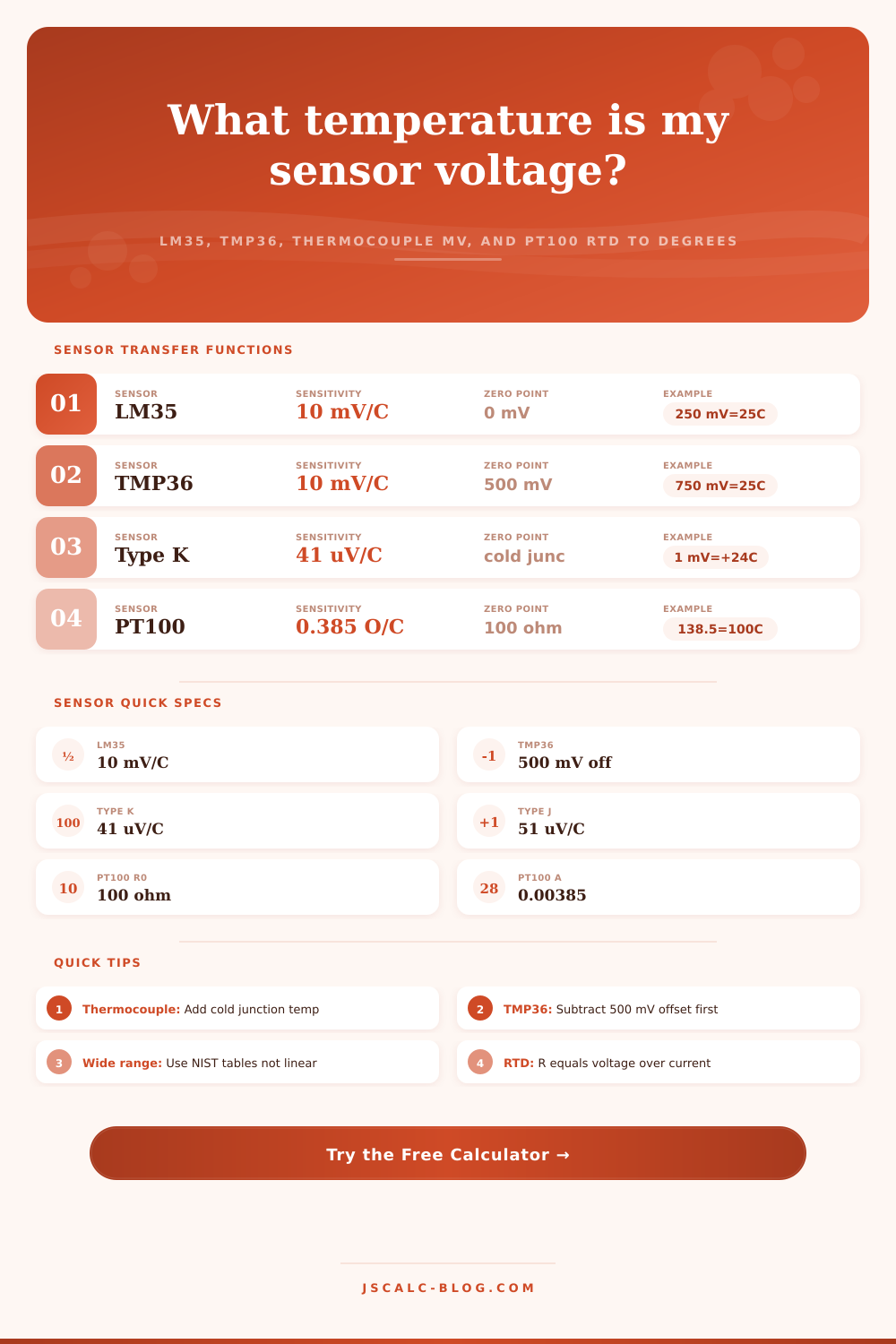
Turn a temperature sensor output voltage into degrees Celsius and Fahrenheit for LM35, TMP36, Type K, J, T, and E thermocouples, and PT100 RTDs using each sensor’s real transfer function.
🎯Real Sensor Presets
📝Sensor and Signal Inputs
For RTD in resistance mode, enter the measured resistance instead.
Thermocouples only – the reference junction temperature to add back.
PT100 voltage mode: R = V / I converts voltage to resistance.
Set to 1 for raw junction voltage. Use amp gain if you read the amplified output.
🔢Sensor Sensitivities
⚡Thermocouple Seebeck Coefficients
| Type | Materials | Seebeck (near 25°C) | Typical Range | Common Use |
|---|---|---|---|---|
| Type K | Chromel / Alumel | 41 µV/°C | –200 to 1260°C | General purpose, ovens |
| Type J | Iron / Constantan | 51 µV/°C | –40 to 750°C | Older equipment, plastics |
| Type T | Copper / Constantan | 43 µV/°C | –200 to 350°C | Cryogenics, food, labs |
| Type E | Chromel / Constantan | 68 µV/°C | –200 to 900°C | High output, low temp |
| Type N | Nicrosil / Nisil | 39 µV/°C | –200 to 1300°C | Stable, high temp |
Seebeck values are near-room-temperature approximations. Thermocouple output is nonlinear across wide spans – use NIST ITS-90 tables or polynomials for accurate wide-range readings.
📊LM35 and TMP36 Voltage Chart
| Temperature | LM35 Output | TMP36 Output | °F |
|---|---|---|---|
| –10°C | –100 mV | 400 mV | 14°F |
| 0°C | 0 mV | 500 mV | 32°F |
| 10°C | 100 mV | 600 mV | 50°F |
| 25°C | 250 mV | 750 mV | 77°F |
| 50°C | 500 mV | 1000 mV | 122°F |
| 85°C | 850 mV | 1350 mV | 185°F |
| 100°C | 1000 mV | 1500 mV | 212°F |
🌡PT100 RTD Resistance vs Temperature
| Temperature | Resistance | V at 1 mA | Notes |
|---|---|---|---|
| –50°C | 80.31 Ω | 80.31 mV | Below ice point |
| 0°C | 100.00 Ω | 100.0 mV | R0 reference |
| 25°C | 109.62 Ω | 109.6 mV | Room temperature |
| 50°C | 119.24 Ω | 119.2 mV | Warm |
| 100°C | 138.51 Ω | 138.5 mV | Water boiling |
| 200°C | 175.86 Ω | 175.9 mV | High heat |
Linear model R = 100(1 + 0.00385 × T). Standard PT100 uses the Callendar–Van Dusen equation for full accuracy, especially above 100°C.
🗂Voltage to Temperature Comparison Grid
| Voltage | LM35 °C | TMP36 °C | Type K °C* | LM35 °F | TMP36 °F |
|---|---|---|---|---|---|
| 0 mV | 0.0 | –50.0 | 25.0 | 32.0 | –58.0 |
| 100 mV | 10.0 | –40.0 | 26.4 | 50.0 | –40.0 |
| 250 mV | 25.0 | –25.0 | 31.1 | 77.0 | –13.0 |
| 500 mV | 50.0 | 0.0 | 37.2 | 122.0 | 32.0 |
| 750 mV | 75.0 | 25.0 | 43.3 | 167.0 | 77.0 |
| 1000 mV | 100.0 | 50.0 | 49.4 | 212.0 | 122.0 |
| 1350 mV | 135.0 | 85.0 | 57.9 | 275.0 | 185.0 |
| 2000 mV | 200.0 | 150.0 | 73.8 | 392.0 | 302.0 |
*Type K column assumes a 25°C cold junction and the 41 µV/°C linear approximation.
⚙Transfer Function Breakdown
💡Practical Conversion Tips
When working with sensors, you wonder, “Is my boiler heating up? Is it overheating?” And you check on it with a multimeter and see a tiny voltage, and you don’t know. That’s one of those common moments when you think: I’m confused! Most measurement error lurk within this gap, the gap between something happening physically, and its electrical signal. Most of the time, it’s not bad hardware. Most of the time, it’s some forgotten reference point, some overlooked offset. You close that gap when you understand how voltage maps onto reality for your particular device.
The reason that analog integrated circuits such as TMP36 and LM35 are so popular is that they make the math easy: simple arithmetic. With the LM35, you get ten millivolts per degree celsius, and it outputs zero volts at zero degrees. It is straightforward ratiometric scaling: divide by ten and there is your temperature. The TMP36 has the same sensitivity, but it provides a five hundred millivolt offset so that it measures below freezing without going negative voltage territory.
How to Understand Sensor Voltage Readings
That’s where folks goes wrong; that offset is what you need to subtract out first before you do the division by ten. Otherwise, you’ll think something’s gone horribly wrong when your room temperature read more like a freezer failure. By selecting the proper sensor type in the dropdown box, the calculator above will perform that subtraction for you automaticly (so you don’t have to do the mental arithmetic when trouble-shooting late at night).
Thermocouples are another matter entirely. Thermocouples work based off different physics and need careful handling. They don’t actualy measure temperature. They measure potential difference created by the Seebeck effect across the junction of two dissimilar metals. For example, a Type K thermocouple generates about forty-one microvolts/°C at around room temperature. This is small enough that without care you will swamp this voltage with noise from your wiring. It only tells you how hot the measurement junction is compared to the reference junction, where your wires join and connect to your instruments.
So if your input terminals are at twenty-five degrees Celsius and you read a voltage that equates to ten degrees difference then the true temperature is thirty-five degrees. You cannot get away without adding that cold junction compensation if you want accuracy.
Another solution comes from Resistance Temperature Detectors which are simply predictable devices that exhibit a change in electrical resistance as a function of temperature. Specifically, for a PT100 type sensor, the resistance is 100 ohms at zero degrees Celsius. It increase predictably by a factor of 0.000385 per each degree so if you pass a small current (excitation) through the sensor and then measure the voltage drop across it with Ohm’s Law, you’ll have a voltage measurement.
You can enter either the calculated resistance or the raw voltage into the calculator, making it flexible based on whether your bridge circuit outputs voltage or resistance. Some do both; one will give you a resistance value and the other will provide a millivolt drop. Either way works but selecting the correct mode means you don’t count conversions twice.
If a relationship isn’t linear, how do you know when to use it? For most hobbyist applications, and for general rough monitoring around room temperature, we can treat the relationship as a straight line. This is not true at extremes of heat or cold; as temperatures approaches extreme heats or cryogenic ranges, the curves bend, making thermocouple outputs non-linear enough to fail simple division. At those extremes, RTDs needs more complex polynomial equations such as Callendar-Van Dusen to stay accurate over broad spans.
The underlying real transfer function is used behind the scenes by the tool, so it will give you correct answers even when a linear model would of been off track. So now instead of voltage readings that confuse you, they become useful information; instead of guessing, you know. You can see how it applies to you and what those numbers represent. Whether it’s a faulty oven calibration or a thermostat troubleshooting session, having the reference points correct realy matters.
The voltage is a messenger. It speaks, but you need to learn its language first.