Trimmed Mean Calculator
Sort a numeric sample, trim the same percentage from each tail, average the retained values, and compare the result with ordinary mean, winsorized mean, and median.
📌 Presets
Load a realistic sample, then adjust values or trim percentage as needed.
Trimmed Mean Result
Sorted sample with matching tails removed.
🧮 Calculator Inputs
📐 Current Comparison Grid
Formula used: sort values, trim floor(n x pct / 100) from each tail, then mean the remaining values.
🗂 Robust Average Comparison
Ordinary Mean
Adds every value and divides by n. It is simple, but one extreme value can pull it hard.
Trimmed Mean
Sorts values, removes the same tail count on both ends, and averages the middle values.
Winsorized Mean
Sorts values and caps the tails at the nearest kept values, so n stays unchanged.
Median
Uses the middle sorted value. It is very resistant to extremes but ignores distances from the center.
📋 Trim Percentage Guide
| Trim per tail | Best fit | Values removed | Use when |
|---|---|---|---|
| 0% | Ordinary mean | None | The sample is clean and extremes are meaningful. |
| 5% | Light robustness | floor(n x 0.05) each side | A few values may be transcription errors or rare spikes. |
| 10% | Common reporting | floor(n x 0.10) each side | You want a central average that still uses most of the sample. |
| 20% | Noisy samples | floor(n x 0.20) each side | Judging panels, surveys, and readings with clear tail noise. |
| 25% | Strong trimming | floor(n x 0.25) each side | The center is more important than preserving tail detail. |
| 49% max | Near median | Must leave at least one value | Only for sensitivity checks; most reports use lower trim levels. |
📊 Worked Reference Table
| Sample | n | Trim | Tail count | Kept count | Why use it |
|---|---|---|---|---|---|
| Seven test scores | 7 | 10% | 0 each side | 7 | floor(7 x 0.10) is 0, so no trimming happens. |
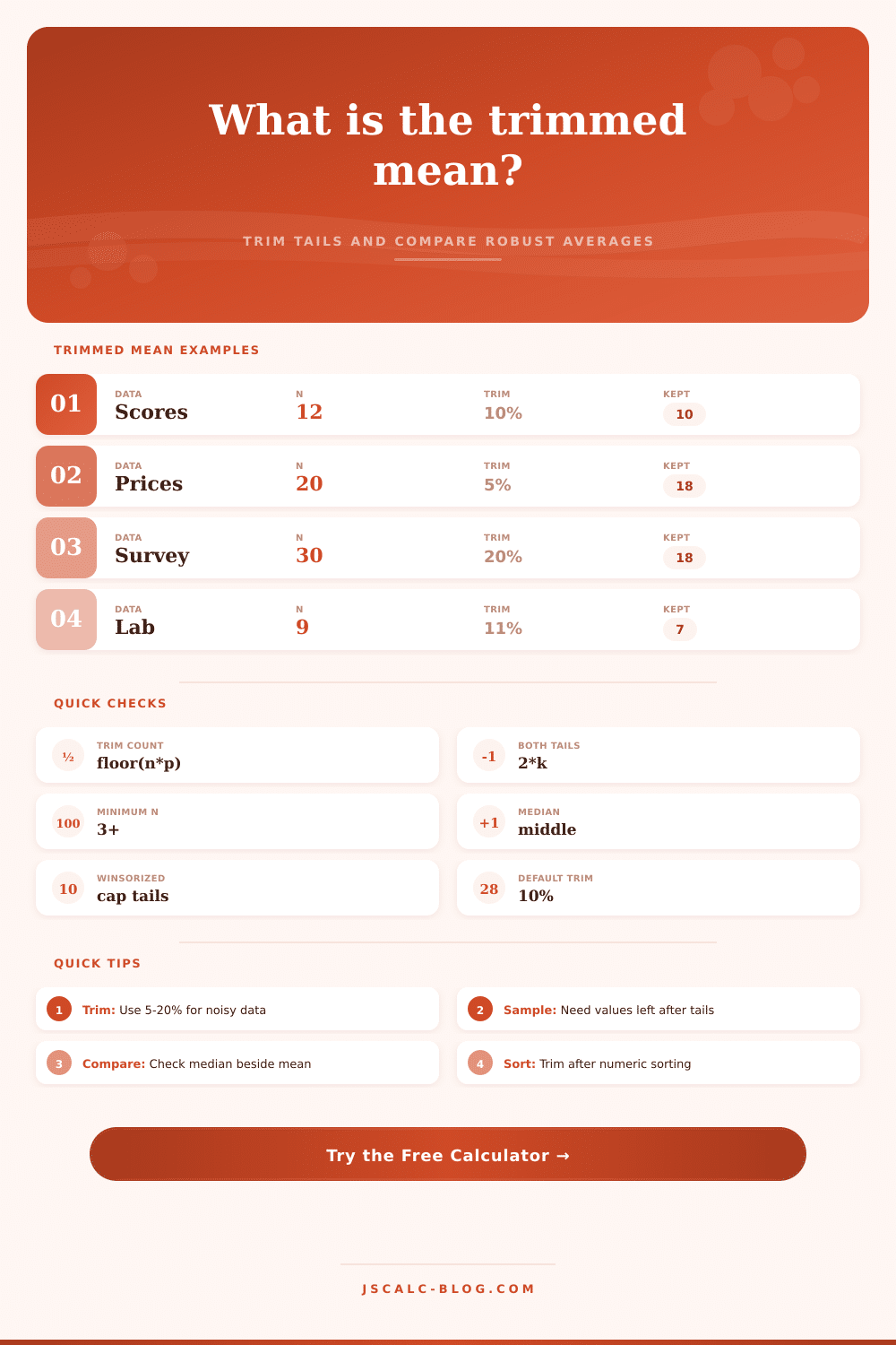
| Twelve judged scores | 12 | 10% | 1 each side | 10 | One high and one low score are removed before averaging. |
| Twenty wait times | 20 | 5% | 1 each side | 18 | Light trimming protects the mean from single unusual waits. |
| Thirty survey values | 30 | 20% | 6 each side | 18 | Heavy trimming focuses on the middle respondent group. |
| Nine lab replicates | 9 | 11% | 0 each side | 9 | Because floor(9 x 0.11) is 0, increase trim to remove tails. |
| Forty daily errors | 40 | 15% | 6 each side | 28 | A larger sample can support more tail removal. |
🧭 Robust Averaging Method Table
| Method | Tail handling | Sample size used | Best use | Main caution |
|---|---|---|---|---|
| Ordinary mean | Keeps every value | All n values | Clean data where extremes are valid measurements. | One outlier can shift the result a lot. |
| Trimmed mean | Removes equal low and high tail counts | n minus 2k | Robust reporting for scores, surveys, waits, and noisy readings. | Small samples may trim nothing because k uses floor(). |
| Winsorized mean | Caps tails at nearest kept values | All n values | Comparing tail influence while preserving the original count. | Capped values are adjusted, so report the cap rule clearly. |
| Median | Uses the sorted middle only | One or two center values | Very skewed data or quick resistance to extreme values. | It ignores how tightly the center values cluster. |
| Interquartile mean | Keeps the middle 50% | About n / 2 | Heavy-tail checks when quartile behavior matters. | It discards more data than a common 10% trim. |
| Midhinge | Averages Q1 and Q3 | Quartile positions | Quick center estimate from a five-number summary. | It is a summary shortcut, not a full-sample average. |
💡 Tips
This means you will see, for instance, that averaging your customers’ ratings may skew results if one angry customer drags rating down from a solid four stars to a concerning three. Your overall rating could drop from 4/5 stars to 3/5 because of this outlier. This isn’t a fault in the calculation, necessarily, just that it doesn’t represent what most people’s experiences is like. The standard mean treats all points equally and is fine as long as your data is fairly clean (i.e., not too many outliers), but if you have some extreme value, the trimmed mean solves that issue. Essentially, it excludes the outliers first and then calculates its center.
With the calculator up there, you can do math yourself, but knowing how and why trimming help also matters. In practice, it’s easy, but there is some precise steps here. First, you take your dataset, arrange it low-to-high, slice off an equal percentage at each end. It’s symmetric. Slice 10% off the top; slice 10% off the bottom. Then calculate mean of what’s left.
How the Trimmed Mean Works
It sounds like throwing away information, but that’s not true: you’re throwing away noise. It’s deciding between what’s the mathematically perfect middle versus what’s the usual experience. Those aren’t always different than the same thing. The biggest variable is how much you trim (trim percentage). Depending on your data, this will make or break it.
At the low end, trimming at five percent will remove only those values that are far outside the norm. This is good if you know there’s some random error in your data. At high end, trimming at twenty percent will start to focus in on meat of the data. This is typical when you’re trying to get past the really skilled player and really bad player in a competition: take out all the strict and lenient judges.
In practice, the calculator floors value for small samples. So, if you’re trimming off ten percent and you’ve got only seven items, it’ll round down to zero, which means nothing gets thrown away. It takes a decent size sample for the trim do anything.
You can get even more insight by comparing different results. For example, the tool will show you the winsorized mean and the trimmed mean. The winsorized mean caps out the extreme values to the next closest kept value (without trimming it). In this way, the winsorized mean doesn’t remove any values but lowers the impact that outliers has on your mean. By looking at how similar these two means are, you can see if your data has been influenced by outliers or not. It’s like a check on distribution of your data. You’re not only getting a number, but you’re assessing quality of your data.
Just for comparison’s sake, we’ve added the median as well. While the median isn’t swayed by extreme numbers, it doesn’t take into account how far away the remaining values are from the median. Between the median and the standard mean lies the trimmed mean, which considers distance from the mean but guards against outliers. In a lot of reports, that’s a nice balance. Take into account everything you have, but don’t let the extremes skew your results.
The real world isn’t perfect. Sensors can drift. Surveys might have missing answers. You account for this with a strong average. Rather than assuming an ideal distribution, you acknowledge the variability and pick a measure that takes it into account.
The page presents a reference table showing which values get dropped and kept at various levels of trimming for different sample sizes. It translates percents into actualy numbers. Now you know exactly what gets cut out in service of clarity. You want to point out trends, not cover up mistakes.
If it’s quiet, you can hear the music. If there’s less noise, you see what’s going on. With the trimmed mean, you show a solid central tendency. One terrible day won’t overwhelm your month of great days. It lets you compare apples-to-apples. What’s left is your run-of-the-mill number. It is your typical experience. It is an average that stands up when looked at closely. It is something grounded in the real world.
The math backs up the narrative. It is a narrative that doesn’t make you think twice. You should of used it more often.