Signal to Noise Ratio Calculator
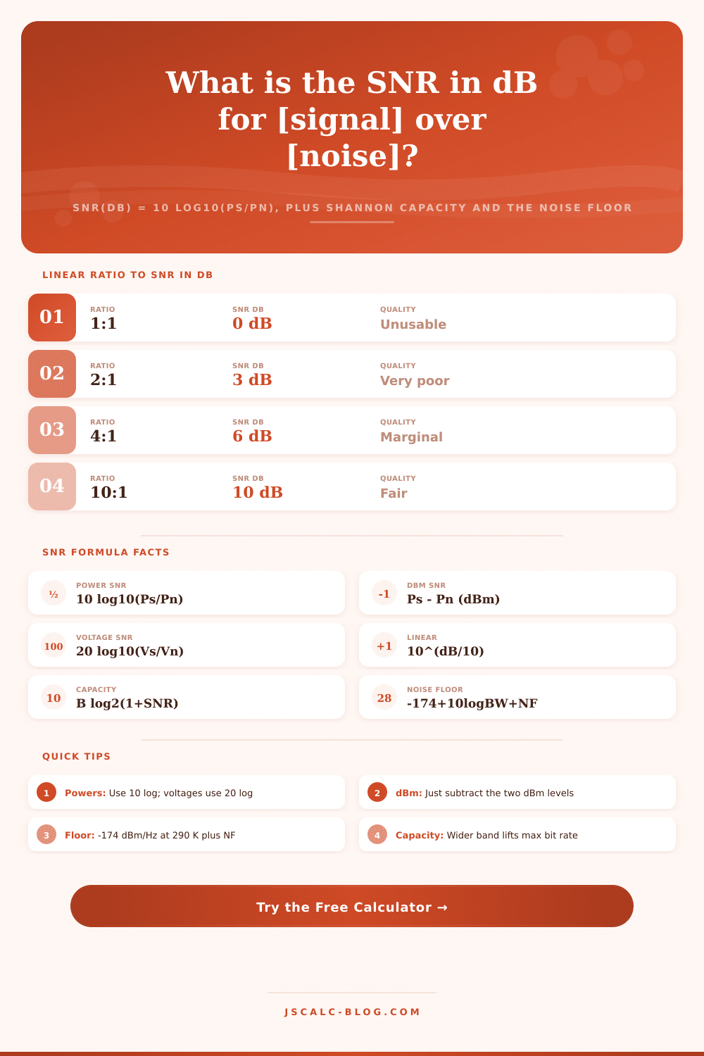
Find the signal to noise ratio in decibels from raw powers, from dBm levels, or from voltage amplitudes, then read the linear SNR, the Shannon-Hartley channel capacity for a given bandwidth, and the thermal noise floor set by kTB at 290 K and your receiver noise figure.
🔊Choose an Input Mode
📡Real-World SNR Presets
📝Signal and Noise Inputs
Average signal power in the unit chosen below.
Total in-band noise power, same unit as signal.
Applies to both power fields above.
Received signal strength in dBm.
Noise floor in dBm; SNR is the difference.
RMS signal amplitude across a fixed impedance.
RMS noise amplitude; voltages use 20 log10.
Shannon mode: enter SNR directly to size capacity.
Channel or noise bandwidth for capacity and floor.
Applies to the bandwidth field above.
Added to the -174 dBm/Hz thermal floor.
Controls rounding on every result card.
🔢Formula Snapshot
📊Linear Ratio to Decibel Reference
| Power Ratio Ps:Pn | SNR in dB (10 log) | Voltage Ratio Vs:Vn | Link Quality |
|---|---|---|---|
| 1 : 1 | 0 dB | 1 : 1 | Unusable, buried |
| 2 : 1 | 3.01 dB | 1.41 : 1 | Very poor |
| 4 : 1 | 6.02 dB | 2 : 1 | Marginal |
| 10 : 1 | 10 dB | 3.16 : 1 | Fair, decodable |
| 100 : 1 | 20 dB | 10 : 1 | Good data link |
| 1000 : 1 | 30 dB | 31.6 : 1 | Great, robust |
| 10000 : 1 | 40 dB | 100 : 1 | Clean channel |
| 1000000 : 1 | 60 dB | 1000 : 1 | Excellent, hi-fi |
🎵Typical System SNR Benchmarks
| System | Typical SNR | Dominant Noise | Notes |
|---|---|---|---|
| CD digital audio | 96 dB | Quantization | 16-bit, 6.02 x 16 |
| 24-bit studio ADC | 120-144 dB | Thermal / dither | Approx 6.02 x N |
| Vinyl LP record | 55-65 dB | Surface hiss | Groove and wear |
| FM broadcast | 50-70 dB | Receiver front end | After de-emphasis |
| Wi-Fi usable link | 20-40 dB | Co-channel | 25 dB for 64-QAM |
| LTE cell edge | 0-10 dB | Interference | Down to -6 dB SNR |
| GPS at antenna | -20 dB | Thermal noise | Recovered by code gain |
📡Thermal Noise Floor by Bandwidth
| Bandwidth | 10 log(BW) | Floor at NF 0 dB | Floor at NF 3 dB | Floor at NF 6 dB |
|---|---|---|---|---|
| 1 Hz | 0 dB | -174 dBm | -171 dBm | -168 dBm |
| 1 kHz | 30 dB | -144 dBm | -141 dBm | -138 dBm |
| 200 kHz | 53 dB | -121 dBm | -118 dBm | -115 dBm |
| 1 MHz | 60 dB | -114 dBm | -111 dBm | -108 dBm |
| 20 MHz | 73 dB | -101 dBm | -98 dBm | -95 dBm |
| 100 MHz | 80 dB | -94 dBm | -91 dBm | -88 dBm |
📏SNR and Voltage Unit Conversions
| Quantity | Formula | Example In | Result |
|---|---|---|---|
| Linear from dB | 10^(dB/10) | 20 dB | 100 x power |
| dB from linear | 10 log10(ratio) | 1000 x | 30 dB |
| Voltage ratio | 10^(dB/20) | 40 dB | 100 x voltage |
| ENOB from SNR | (SNR - 1.76)/6.02 | 74 dB | 12 bits |
| dBm to mW | 10^(dBm/10) | 0 dBm | 1 mW |
| Half power | ratio 0.5 | -3.01 dB | 50% power |
🗃Shannon Capacity Comparison Grid
| Bandwidth | SNR dB | Linear SNR | log2(1+SNR) | Capacity | Spectral Eff |
|---|---|---|---|---|---|
| 20 MHz | 0 dB | 1 | 1.00 | 20 Mbps | 1.0 b/s/Hz |
| 20 MHz | 10 dB | 10 | 3.46 | 69.2 Mbps | 3.46 b/s/Hz |
| 20 MHz | 20 dB | 100 | 6.66 | 133 Mbps | 6.66 b/s/Hz |
| 20 MHz | 30 dB | 1000 | 9.97 | 199 Mbps | 9.97 b/s/Hz |
| 40 MHz | 25 dB | 316 | 8.31 | 332 Mbps | 8.31 b/s/Hz |
| 1 MHz | 15 dB | 31.6 | 5.03 | 5.03 Mbps | 5.03 b/s/Hz |
| 200 kHz | 9 dB | 7.94 | 3.16 | 632 kbps | 3.16 b/s/Hz |
| 3.1 kHz | 36 dB | 3981 | 11.96 | 37.1 kbps | 11.96 b/s/Hz |
| 100 MHz | 20 dB | 100 | 6.66 | 666 Mbps | 6.66 b/s/Hz |
| 80 MHz | 40 dB | 10000 | 13.29 | 1.06 Gbps | 13.29 b/s/Hz |
⚙Formula Breakdown
💡Practical SNR Tips
Maybe you’ve stood in a room that had only one bar of signal on your phone. Maybe you’ve heard about the signal to noise ratio, it’s not just a matter of how loudly your signal gets out there; it matters what kind of background noise there is too. It turns that idea into real numbers. Switch between voltage levels, decibels or even just raw power levels and see where your link sit without wasting your time (or any money on hardware).
The basic metric are just dividing. Divide the average power in signal in the given bandwidth by the average power of noise in the same bandwidth. In reality these numbers range from one to more than a million. Engineers express this as decibels, which squishes those values down to something we can deal with in two digits. A hundred-to-one ratio are expressed as twenty decibels; a thousand-to-one is expressed as thirty. The calculator do all the log math for you.
How This Calculator Works
You might be thinking that I’m confusing voltage and power inputs. That’s another common trap. It makes it into the equation different: power goes as voltage squared (which is why you use ten times the logarithm for watts but twenty times the logarithm for voltages). If you’re measuring voltage, the number’s 20x; if you’re measuring energy/power, it’s 10x log. You get thrown off by a factor-of-two difference in the exponent if you forget. The interface keep things clean and separate. You choose the proper path based off whether you measured an amount of energy or an amount of amplitude.
But with an SNR number in hand, what do we do next? What does it mean in terms of data capacity? Here, we’re back in 1948, with Claude Shannon’s still-dominant rule over the industry. According to his theorem, Channel Capacity = (Bandwidth) x (Log2(1+LinearSNR)). This means you multiply the bandwidth by the logarithm base two of one plus your signal-to-noise ratio expressed as a linear number. This is where the calculator will take your decibel value and convert it back into a linear ratio, then apply the equation on the fly, displaying the theoretical limit for error-free throughput. In other words, if your signal strength looks great but you feel like your link is laggy anyway, looking at this capacity value frequently will often expose the fact that rather than bandwidth limits, noise is devouring your headroom.
There is thermal noise on a hard floor. Every receiver have a hard floor of thermal noise. Below that, there’s just the random jiggling of electrons in anything warmer than absolute zero (a hiss). That floor is -174 dBm per hertz at room temperature. The tool shows how much it adds to your bandwidth and noise figure as the total absolute minimum noise you’ll experience. Physics can’t be filtered away. Knowing about it help explain why shrinking a receiver’s bandwidth get better performance. It removes irrelevant sources of noise, improving the ratio but not altering signal itself.
The numbers themselves are abstract, though… And that’s where the reference tables on the page come into play. They translate those abstracts into things you know: fifty to sixty decibels sounds like the surface hiss of a vinyl record; ninety-six decibels is the level of a compact disc audio track. Wi-Fi operates at roughly twenty to forty decibels, which is just enough to make it go. GPS signals are frequently lost in noise entirely, relying on advanced processing gain to pull through. Seeing these numbers side by side helps you understand what to realisticly expect in your own environment.
You can see exactly what’s going on in the breakdown section: where all the inputs go and how they calculate to the end result. There is also an effective number of bits figure that shows how much resolution your ADC has by translating the signal-to-noise ratio (SNR). One bit is roughly equal to six decibel signal margin. So if you’re looking at making a sensor interface, this will let you know right away if your amplifier chain are good enough to get the required accuracy.
In short, making a link better is frequently as much about minimizing noise as it is increasing power. You can usually buy a better amplifier but filtering unwanted bandwidth is usually cheaper. If you are up against thermal limitations, cooling parts will help, as will using lower-noise amplifiers. Using this calculator lets you experiment with these tradeoffs in advance so you would of spent money on an expensive mistake. It makes a complex physical problem a clear mathematical one, allowing you to determine whether you want more signal or just to quieten the room down.