Sensitivity and Specificity Calculator
Enter true positives, false negatives, true negatives, and false positives to calculate sensitivity, specificity, likelihood ratios, accuracy, predictive values, and reporting-ready diagnostic checks.
🎯Diagnostic Presets
📝Confusion Matrix Inputs
Name the disease, defect, event, or target class.
Positive test among truly positive cases.
Negative test among truly positive cases.
Negative test among truly negative cases.
Positive test among truly negative cases.
🧮Diagnostic Summary Grid
📊Current 2x2 Diagnostic Table
📐Metric Formula Table
⚖Likelihood Ratio Interpretation
| Metric | Band | Evidence Strength | Typical Meaning | Caution |
|---|---|---|---|---|
| LR+ | 1.0 | None | Positive result does not change odds | Check coding and reference standard |
| LR+ | 2 to 5 | Small to useful | Positive result modestly raises probability | Base rate still matters |
| LR+ | 5 to 10 | Moderate | Positive result is meaningfully persuasive | Verify sample representativeness |
| LR+ | 10+ | Strong | Positive result can be good for rule-in use | Wide intervals need caution |
| LR- | 0.5 to 1 | Weak | Negative result leaves much uncertainty | Misses may remain frequent |
| LR- | 0.2 to 0.5 | Moderate | Negative result lowers probability | Use with clinical context |
| LR- | 0.1 to 0.2 | Strong | Negative result can support rule-out use | Needs reliable sensitivity |
| LR- | Below 0.1 | Very strong | Negative result sharply lowers probability | Confirm external validation |
🔍Preset Benchmark Table
| Preset | TP | FN | TN | FP | Main Read |
|---|---|---|---|---|---|
| Rare disease screen | 92 | 8 | 855 | 45 | Good sensitivity, PPV limited by low prevalence |
| Emergency rule-out | 146 | 4 | 690 | 160 | Excellent sensitivity, many false alarms |
| High specificity rule-in | 108 | 42 | 828 | 22 | Positive results carry stronger rule-in evidence |
| Rapid antigen audit | 240 | 60 | 650 | 50 | Specificity is high, sensitivity is moderate |
| AI triage model | 410 | 90 | 1280 | 220 | Balanced model with visible false-positive load |
| Lab assay validation | 188 | 12 | 776 | 24 | Strong sensitivity and specificity together |
| Factory defect sensor | 64 | 16 | 1840 | 80 | Low prevalence makes PPV sensitive to FP count |
| Veterinary herd test | 210 | 30 | 1470 | 90 | Useful screening pattern for group decisions |
| Screening panel review | 520 | 80 | 3300 | 300 | Large sample shows stable accuracy estimates |
| Small pilot study | 18 | 7 | 62 | 13 | Small denominators need interval reporting |
⚙Full Formula Breakdown
💡Diagnostic Reporting Tips
Educational calculation only. For clinical, regulatory, or operational decisions, validate the reference standard, sampling plan, and intended-use population.
Each diagnostic test you perform is actualy a guessing game, but on partial information. Patient may or may not be ill. The test may or may not be correct. Because of this, the diagnosis you make can affect everything. The problem is that there is this trade off between false alarms and capturing all cases. And no test do that right. In other words, thats the nature of clinical evaluation.
And so to cut through that confusion, you reach for a 2×2 matrix. Yes, its boring. But if it sounds unfamiliar, it’s because it’s foundation of evidence-based medicine.
Understanding Diagnostic Tests
The idea is that you count four things. You count true positives (the patients whose case you called correctly) and false positives (the healthy people you alarmed needlessy). You also count true negatives (the healthy people you cleared correctly) and false negatives (the dangerous misses). Plug the raw number into the calculator above, and math strips out guesswork.
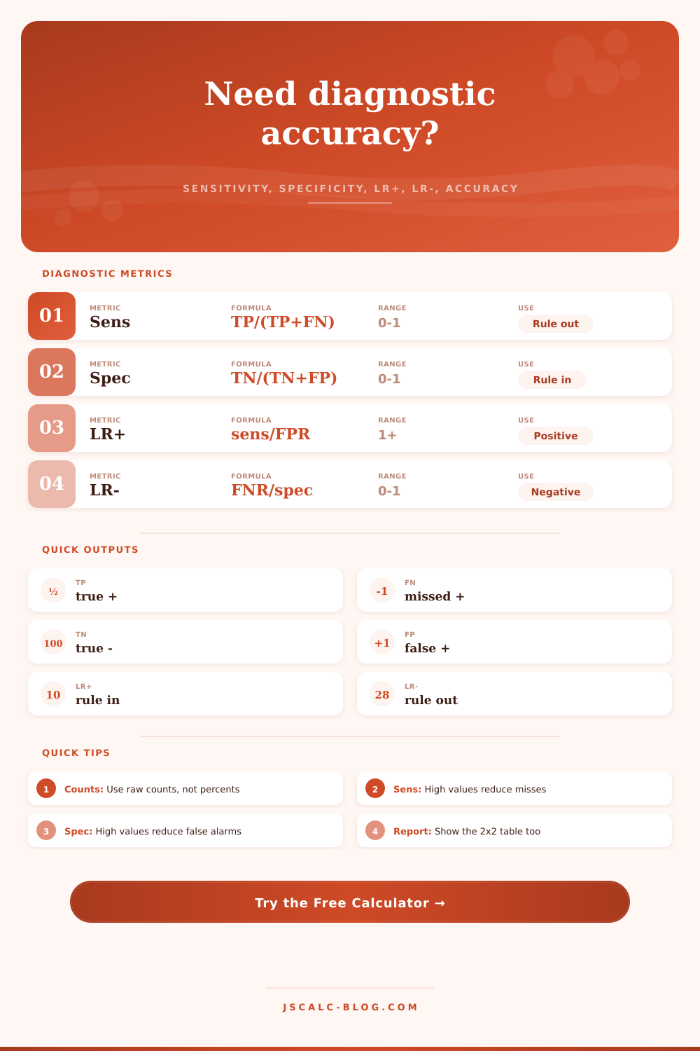
Sensitivity measures how well your test find the disease. Sensitivity is the proportion of actual cases that test positive. If sensitivity is high, this will rarely fails to find anyone with disease, which is important if missing someone would be deadly: you’d want to cast a wide net.
The opposite is what we mean by specificity. How well does the test identifies healthy people? High specificity give you few false alarms. This is important if taking action would be risky/expensive; you want to be sure.
Here’s the trick: it can’t be optimized in both directions simultaneously. If you move the threshold up to capture more of those sick people, then by definition youll also capture more of those who are just healthy. And that’s where people misunderstand; they want a perfect test and there is no such things. It says so right on the page in the reference table, which spells out how different presets manages the trade-offs between the two.
For example, if you’re looking for a screening tool for a rare disease, you want to prioritize sensitivity. If you’re doing a confirmatory test for something that could have serious treatments, you want to prioritize specificity.
Test results don’t directly answer whether a patient has a disease. Instead, they shift our confidence one way or another. Likelihood ratios provides a sharper lens by showing us how much a test result changes things.
If a positive likelihood ratio is high, then a positive result goes a long way toward confirming the diagnosis. If a negative likelihood ratio is low, then a negative result virtually excludes it.
Unlike predictive values, which depend on prevalence of the disease in your particular clinical setting, these likelihood ratios relies solely on the test itself and thus tend to be more stable.
But then there’s prevalence. When something is rare, positive predictive value plummets, even your most specific test will spit out a lot of false positives when nearly everyone tested has no reason to be sick. This is what makes it so that a positive screen for a rare disease is hardly ever conclusive; it only indicates you should of look further.
With negative predictive value, it’s the reverse. The more rare the condition, the higher the negative predictive value. This means a negative test for a rare condition give you very good reassurance.
Noise comes from small samples. If you shrink the size of the denominator, then the confidence interval widens, and the smaller your study (e.g., a 95% sensitive test on 10 patients) become, the less useful it is. It could be anything from 50% to 100%. So here are those intervals that let you look at how certain you should be. Look at their width. The narrower, the better. The bigger, wait until there’s more.
Diagnostics are a mess in the real world. The reference standard isn’t perfect. Sampling bias means that tests will skew based off where they’re done. A test well-validated at a specialized center might fail miserably when used in your primary care clinic (because numbers was based on ideal conditions).
Use the metrics for guidance… Don’t follow them like gospel. You need to decide how much the real world differ from the model.
Finally, a test is only a piece of evidence. A test never provides absolute truth; a test only updates your prior belief. If you understand sensitivity and specificity, you will be able to weigh the evidence correctly. And you will cease thinking in terms of pass/fail. You will begin to see probabilities change, moment by moment, and that’s when the true diagnosis occurs.
The numbers do not say, ‘Do this.’ The numbers say only, ‘This is what you know.’