RAID 10 Capacity Calculator
RAID 10 stripes across mirrored pairs for speed and redundancy at once. Usable capacity is exactly half the raw array, computed as the number of drives divided by two times the smallest drive size. Enter your drive count, per-drive size, and drive type to see usable space in TB and TiB, read and write throughput, and how many disk failures the array can survive.
⚡Real RAID 10 Build Presets
💾RAID 10 Array Inputs
Total physical disks. RAID 10 needs an even count.
Size of one disk; use the smallest if mixed.
Applies to the per-drive capacity field.
Sets the default single-drive throughput.
Auto-filled by drive type; override if known.
Per-disk chunk before moving to the next drive.
Number of two-disk mirrors striped together.
Trims formatted space for the metadata card.
🔢RAID 10 Snapshot
📊Usable Capacity by Array Size
| Drives | Mirrored Pairs | Per Drive | Usable (n/2 x size) | Efficiency |
|---|---|---|---|---|
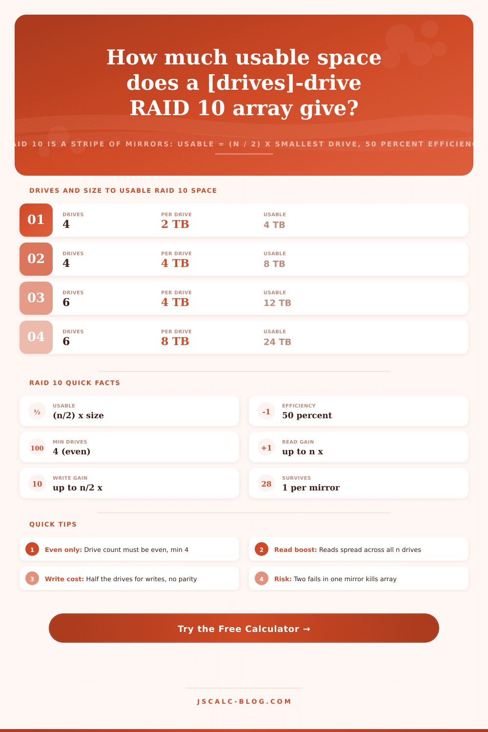
| 4 | 2 | 2 TB | 4 TB | 50% |
| 4 | 2 | 4 TB | 8 TB | 50% |
| 6 | 3 | 4 TB | 12 TB | 50% |
| 6 | 3 | 8 TB | 24 TB | 50% |
| 8 | 4 | 1 TB | 4 TB | 50% |
| 8 | 4 | 4 TB | 16 TB | 50% |
| 10 | 5 | 6 TB | 30 TB | 50% |
| 12 | 6 | 8 TB | 48 TB | 50% |
| 16 | 8 | 4 TB | 32 TB | 50% |
📡Throughput Scaling by Drive Type
| Drive Type | Per Drive | 8-Drive Read | 8-Drive Write | Notes |
|---|---|---|---|---|
| 5400 RPM HDD | 160 MB/s | 1280 MB/s | 640 MB/s | Cool, quiet bulk |
| 7200 RPM HDD | 250 MB/s | 2000 MB/s | 1000 MB/s | NAS workhorse |
| SATA SSD | 550 MB/s | 4400 MB/s | 2200 MB/s | SATA bus limited |
| NVMe SSD | 3500 MB/s | 28000 MB/s | 14000 MB/s | Controller bound |
🗃RAID Level Comparison Grid
| RAID Level | Efficiency | Min Drives | Fault Tolerance | Read Gain | Write Gain |
|---|---|---|---|---|---|
| RAID 0 | 100% | 2 | 0 drives | n x | n x |
| RAID 1 | 50% | 2 | 1 per mirror | up to n x | 1 x |
| RAID 5 | (n-1)/n | 3 | 1 drive | (n-1) x | low, parity |
| RAID 6 | (n-2)/n | 4 | 2 drives | (n-2) x | lower, 2 parity |
| RAID 10 | 50% | 4 | 1 per mirror | up to n x | n/2 x |
| RAID 50 | varies | 6 | 1 per group | high | medium |
| RAID 60 | varies | 8 | 2 per group | high | medium |
🛡Fault Tolerance Scenarios
| Drives | Pairs | Guaranteed Survive | Best Case | Fatal Case |
|---|---|---|---|---|
| 4 | 2 | 1 drive | 2 (1 per pair) | 2 in one pair |
| 6 | 3 | 1 drive | 3 (1 per pair) | 2 in one pair |
| 8 | 4 | 1 drive | 4 (1 per pair) | 2 in one pair |
| 10 | 5 | 1 drive | 5 (1 per pair) | 2 in one pair |
| 12 | 6 | 1 drive | 6 (1 per pair) | 2 in one pair |
| 16 | 8 | 1 drive | 8 (1 per pair) | 2 in one pair |
⚙Formula Breakdown
💡RAID 10 Planning Tips
This leads us to RAID 10, which is an arrangement of storage that’s built on top of two more basic ideas: mirroring (a complete copy of each block of data) and striping (the distribution of that data across several disks). When you stripe across mirrors, you get fast read/write speeds while also retaining the ability to swap out drives without loss of data.
There’s a catch. Because you’re maintaining two separate copies of everything, only half of your available disks are actualy usable. For example, if you have four drives in a RAID 10 array, it act like you have just two. That’s a steep price for some pretty serious speed.
How RAID 10 Works
It’s also rigid in its structure. By design, it begins with an even number of drive (at least four). Then, it takes half of them as a pair and makes that pair a mirror of itself. In other words, for four drives, you get two mirrored sets of four drives; for eight drives, you get four mirrored sets of two drives. Each of these disks contains the same data. Finally, it writes each piece of data to different sets of those mirrors, one to the first pair, the next to the second, etc. Since all the pairs is redundant, that redundancy simply gets carried over to the striped set automatically.
Enter how many and what size drives you want, and the calculator does the rest. It will spare you from having to divide by two in your head or trying to remember where you’re supposed to add parity bits. The 50 percent efficiency rule is important for usable capacity. It is one of the cleanest rules for storing stuff. Divide the number of drives by two and then multiply by the size of the smallest drive. That is sixteen terabytes on eight four-terabyte drives.
Adding more drives does not change efficiency; all the bytes gets written twice so it doesn’t matter how many drives you have. Mismatched drives? Each array size matches the smallest disk. So whatever the weakest link, that’s what determines the speed of the entire array. That keeps the blocks evenly allocated to prevent corruption off the data.
Where RAID 10 stands out and excels, far more than RAID 5 or 6, is in performance. In both mirrored copies, the controller can pull from either copy on a read. So on reads, it has all the drives pulling in parallel. Peak read performance increases towards the speed of one drive times the number of drives. With eight 7200 RPM disks reading sequentially at around 250 megabytes per second each, you can get up to around two gigabytes per second.
Because each block hits both disks in its pair, only half the spindles act as independent write streams during writes. Write throughput scales towards the number of pairs times single-drive speed. And most importantly: no parity computation. That write penalty that slows down parity arrays is avoided. Random write performance remains excellent for virtual machines and databases; indeed, that’s why RAID 10 is popular with those kinds of workloads.
However, there’s a limit on fault tolerance that you need to be aware of. Because you’ve got the mirror copy still serving data while you swap out the dead disk, the array will continue to function even after one drive dies. Best case, many more. However, as long as the failed drives are not all in the same mirror, you can lose up to half the drives without losing the array. You could theoreticly have a sixteen-drive array with eight drives simultaneously dying and it’d keep ticking over provided they’re all perfectly distributed across different mirrors.
That brings us to the worst case… Which is the fatal case. Both disks from the same mirror pair going down means you lost that stripe, and you’ve lost the entire array. Hence, RAID 10 survives one drive per mirror, not a set number overall.
But what are the trade offs? And how do they compare to other levels? Against RAID 0, you gain some redundancy (you lose half your capacity though), whereas plain striping lacks it. Compared to RAID 1, you keep the same level of redundancy but add striping, so performance increases based on the number of drives. Compared to parity levels such as RAID 5 and 6, you use capacity much more efficiently. However, this comes at a high cost in rebuild time because all the drives must recalculate parity after each failure. It also causes a large drop in write performance.
RAID 10 copies over the survivor from a pair onto a new disk. This doesn’t put much stress on the array and takes place quickly.
Drives: Choosing drives sets your performance ceiling. SATA SSDs multiply throughput until the bus limits them. NVMe SSDs are so fast that they push aggregate numbers so high that the controller is now the bottleneck, not the drives. The choice of drive determines your performance. Bulk media stays cool at slower speeds (5400 RPM). Classic NAS workhorses have faster 7200 RPM disks.
Stripes: How many disks does this data land on before it moves to another? The stripe size controls this. Large stripes favor large sequential files (i.e. Video). Small ones can benefit random.
That’s right, it has a bunch of presets that include typical builds ranging from a four-drive setup to a sixteen drive SQL farm. Pick the one nearest to your build, tweak the variables and read off the cards: usable capacity, fault tolerance, read speed, write speed. The idea is the same whether it’s building an enterprise array or a home NAS; know how much half your disks buy you before buying hardware.
You should of paid a 50 percent tax in capacity every time it comes up. And that knowledge is worth the cost.