Protein Molarity Calculator
Convert a protein concentration in mg/mL into molarity as µM and nM using the molecular weight in kDa or Da. Enter a value directly or use an A280 absorbance reading with an extinction coefficient, and see the moles present in a chosen volume.
🧪Real Protein Presets
📝Protein Sample Inputs
Switch to A280 to derive mg/mL from a spectrophotometer reading.
1 mg/mL equals 1 g/L, the basis for the molarity step.
Blank-corrected absorbance at 280 nm.
A280 of a 1 mg/mL solution; BSA is about 0.667.
Standard cuvette is 1 cm; NanoDrop uses 0.1 cm.
Enter the protein mass; unit is set on the right.
1 kDa = 1000 Da = 1000 g/mol.
Large proteins usually land in µM or nM.
Used to report total moles and mass in the tube.
🔢Formula Snapshot
🧬Common Protein Molecular Weights
| Protein | MW (kDa) | MW (Da) | µM at 1 mg/mL |
|---|---|---|---|
| Insulin (monomer) | 5.8 | 5,808 | 172.2 µM |
| Lysozyme | 14.3 | 14,300 | 69.9 µM |
| Trypsin | 23.3 | 23,300 | 42.9 µM |
| GFP | 27.0 | 26,900 | 37.2 µM |
| Streptavidin (tetramer) | 52.8 | 52,800 | 18.9 µM |
| Hemoglobin (tetramer) | 64.5 | 64,500 | 15.5 µM |
| Serum albumin | 66.0 | 66,000 | 15.2 µM |
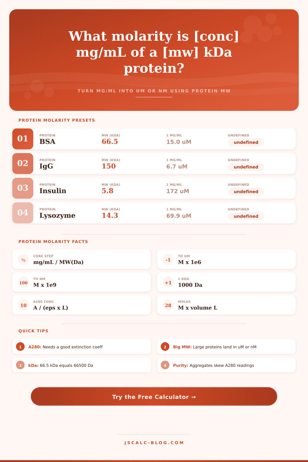
| BSA | 66.5 | 66,500 | 15.0 µM |
| IgG antibody | 150.0 | 150,000 | 6.7 µM |
📊1 mg/mL to Molarity by Molecular Weight
| MW (kDa) | MW (Da) | Molarity at 1 mg/mL | In nM |
|---|---|---|---|
| 5 | 5,000 | 200.0 µM | 200,000 nM |
| 10 | 10,000 | 100.0 µM | 100,000 nM |
| 25 | 25,000 | 40.0 µM | 40,000 nM |
| 50 | 50,000 | 20.0 µM | 20,000 nM |
| 66.5 | 66,500 | 15.0 µM | 15,038 nM |
| 100 | 100,000 | 10.0 µM | 10,000 nM |
| 150 | 150,000 | 6.7 µM | 6,667 nM |
| 250 | 250,000 | 4.0 µM | 4,000 nM |
📏Molarity Unit Conversions
| Unit | Relative to Molar | 1 M equals | Typical protein use |
|---|---|---|---|
| Molar (M) | 1 | 1 M | Rare for proteins |
| Millimolar (mM) | 1e-3 | 1,000 mM | Very concentrated stocks |
| Micromolar (µM) | 1e-6 | 1,000,000 µM | Common working range |
| Nanomolar (nM) | 1e-9 | 1e9 nM | Assays and dilutions |
| Picomolar (pM) | 1e-12 | 1e12 pM | High-affinity binding |
🔬Extinction Coefficient Examples (A280)
| Protein | 0.1% (mL/mg/cm) | Molar ε (M⁻¹cm⁻¹) | Note |
|---|---|---|---|
| BSA | 0.667 | 43,824 | A280 of 1 mg/mL ≈ 0.667 |
| IgG (typical) | 1.40 | 210,000 | Common antibody default |
| Lysozyme | 2.64 | 37,750 | Tryptophan rich |
| GFP | 0.80 | 21,500 | Varies by variant |
| Generic estimate | 1.00 | ≈ MW | Rough fallback only |
🖥Molarity Comparison Grid (µM by mg/mL)
| Protein | MW (kDa) | 0.5 mg/mL | 1 mg/mL | 2 mg/mL | 5 mg/mL |
|---|---|---|---|---|---|
| Insulin | 5.8 | 86.2 µM | 172.4 µM | 344.8 µM | 862.1 µM |
| Lysozyme | 14.3 | 35.0 µM | 69.9 µM | 139.9 µM | 349.7 µM |
| Trypsin | 23.3 | 21.5 µM | 42.9 µM | 85.8 µM | 214.6 µM |
| GFP | 27.0 | 18.5 µM | 37.0 µM | 74.1 µM | 185.2 µM |
| Streptavidin | 52.8 | 9.5 µM | 18.9 µM | 37.9 µM | 94.7 µM |
| Hemoglobin | 64.5 | 7.8 µM | 15.5 µM | 31.0 µM | 77.5 µM |
| BSA | 66.5 | 7.5 µM | 15.0 µM | 30.1 µM | 75.2 µM |
| Albumin | 66.0 | 7.6 µM | 15.2 µM | 30.3 µM | 75.8 µM |
| IgG antibody | 150.0 | 3.3 µM | 6.7 µM | 13.3 µM | 33.3 µM |
⚙Full Formula Breakdown
📋Factor and Basis Reference
| Item | Value | Where It Applies | Effect on Molarity |
|---|---|---|---|
| kDa to Da | × 1000 | MW unit conversion | Sets the divisor size |
| mg/mL to g/L | × 1 | Concentration basis | Direct, no scaling |
| mol/L to µM | × 1e6 | Reporting units | Shifts to micromolar |
| mol/L to nM | × 1e9 | Reporting units | Shifts to nanomolar |
| A280 basis | A ÷ (ε × L) | Absorbance input | Feeds the mg/mL term |
💡Practical Protein Molarity Tips
The molarity of proteins becomes abstract until you’re facing a cuvette with some material in it and you see that one milligram per milliliter doesn’t mean the same thing when it’s insulin as when it’s an antibody. You weighed the same amount, yes, but depending on how heavy each molecule was there could be vastly more or fewer molecules in your tube. That is what causes most lab notebooks to become a mess.
The protein molarity calculator above takes care of translating your unclear mg/mL measurement into a real nanomolar or micromolar figure to plug into your enzyme kinetics or binding assays. What makes this conversion relevant is also what makes it important, scaling.
Why Protein Molarity Is Different From Weight
Glucose is a small molecule. Its molecular weight isn’t very high, and thus its molarity is quite large at relatively small masses. Proteins, however, are huge. Bovine serum albumin is around 66.5 kilodaltons. That seems fine until you start doing some division with the standard mass concentration of 1 mg/mL. You get ~15 micromolar. If you go with an IgG antibody, which hovers around 150 kDa, you gets just 6.7 micromolar at the same mass concentration.
Why? Because we’re talking about proteins here. And when bench scientists discuss proteins, they do so in nanomolars and micromolars, numbers too small to write out as straight-up decimals without looking absurd. That’s how proteins naturaly exist in chemistry, which is why those scales are the defaults on the tool.
Once you ignore the unit confusion, the math gets deceivingly simple. Moles per liter is the same as moles/liter, which is Molarity. Grams per liter is the same as mg/mL (as in protein work). Grams per mole equals Daltons, which are numerically the same thing. So you just divide your mass concentration by your molecular weight in daltons. Multiply that answer by a million and you have micromolar. It is easy. You can use a calculator to do it for you immediately, but knowing how it works helps you find mistakes if the result seems wrong.
If your protein is really big then the molarity will be small. If it’s tiny, like insulin at 5.8 kDa, then one mg/mL becomes almost 172 micromolar. This means you need more dilution buffer so your sample won’t either crash out of solution or saturate your detector.
Instead of balancing, many labs take an absorbance reading at 280 nanometer wavelength and go straight from there. Fortunately, the tool can accommodate this workflow. Here, you input your protein’s extinction coefficient. You also input the absorbance reading and the path length (in micrometers or centimeters) of your microvolume or cuvette instrument. For example, BSA’s extinction coefficient is approximately 0.667 mL/mg/cm. That means if you measure 0.667 in a one centimeter path then you are at one mg/mL. From there, the calculator takes your light absorption measurement to compute the concentration. It then converts that concentration into molarity. It involves one less step and less chance for rounding errors.
More importantly, it forces you to deal with the extinction coefficient which is where most mistakes happen. It’s dangerous to use a generic extinction coefficient. When you don’t have any sequence information, 1.0 is a popular default choice, but it could of being off by twenty or thirty percent for certain proteins, such as one containing lots of tryptophans (lysozyme). Unless you have sequence info available, always get the specific coefficient from an online sequence analysis tool.
There’s also this other twist: aggregation. Proteins that stick together alter their apparent molecular weight, making your molarity calculation useless. The protein must be assumed to be uniform (not aggregated) and pure in solution. How does the calculator know that? It doesn’t. That’s what you’re there for. Run a gel, or at least check your absorbance ratio if the numbers look fishy.
For example, the tool includes preset buttons for common reagents like GFP and streptavidin. These allow you to quickly see what volume of each protein size is needed to reach a certain molarity. And, because bigger proteins has higher molecular weight than smaller ones, they require larger volumes at any given molarity. When you’re titrating a binding partner, you don’t want equal masses; you want equal molar amounts. The moles per volume field links the pipette to the spectrophotometer by calculating exactly how many picomoles are in your twenty microliter aliquot.
In part, working with proteins is all about scale. There are far more molecules in a milligram of hemoglobin than there are in a milligram of insulin. The calculator helps take away the math friction so that you can focus instead on whether or not your concentrations makes sense given the context of your experiment. Bookmark the page and use it as an insurance check to double-check your dilutions before you commit some of your precious reagent to a plate. It’s a little thing, but getting the molarity right is often what makes the difference between background noise and a clear signal.