Power for a T-Test Calculator

Estimate statistical power for one-sample, paired, equal-size two-sample, and unequal two-sample t-tests. Enter the mean shift or Cohen's d, sample sizes, alpha, and tail direction to see effect size, noncentrality, critical t, and the probability of rejection under the alternative.

🎯Real Study Presets

📝T-Test Power Inputs

T-test design

Alternative and rejection tail

Significance level alpha

Common choices are 0.05, 0.01, and 0.10.

Effect size entry method

Reference or control mean

For paired tests, enter the null mean difference, usually 0.

Expected treatment mean or difference

The signed direction matters for one-tailed power.

Standard deviation or pooled SD

Use SD of paired differences for paired designs.

Sample size plan n or n1,n2

Enter 34 for one/paired/equal groups, or 120,80 for unequal two-sample.

Estimated power 0% P(reject H0 | alternative)

Effect size d 0.00 (mean shift) / SD

Noncentrality 0.00 d times design sample term

Critical t 0.00 alpha cutoff with df

🔢Power Snapshot

33Degrees freedom

1.71Standard error

34Approx n for 80%

NCTApprox method

📊T-Test Design Comparison Grid

Design	Effect Size d	Noncentrality	Degrees Freedom	Best Input SD	Use Case
One-sample	(mu1 - mu0) / sigma	d x sqrt(n)	n - 1	Outcome SD	Single group vs benchmark
Paired	Mean diff / SD diff	d x sqrt(n)	n - 1	Within-pair difference SD	Before/after or matched pairs
Two-sample equal n	(mu1 - mu0) / pooled SD	d x sqrt(n/2)	2n - 2	Pooled group SD	Balanced treatment/control
Two-sample unequal n	(mu1 - mu0) / pooled SD	d x sqrt(n1 x n2 / (n1+n2))	n1 + n2 - 2	Pooled group SD	Allocation constrained study

📐Common Power Benchmarks

Scenario	Design	Effect d	Alpha	Target	Approx Sample Size
Small effect screen	One-sample	0.20	0.05 two-sided	80%	About 197 total
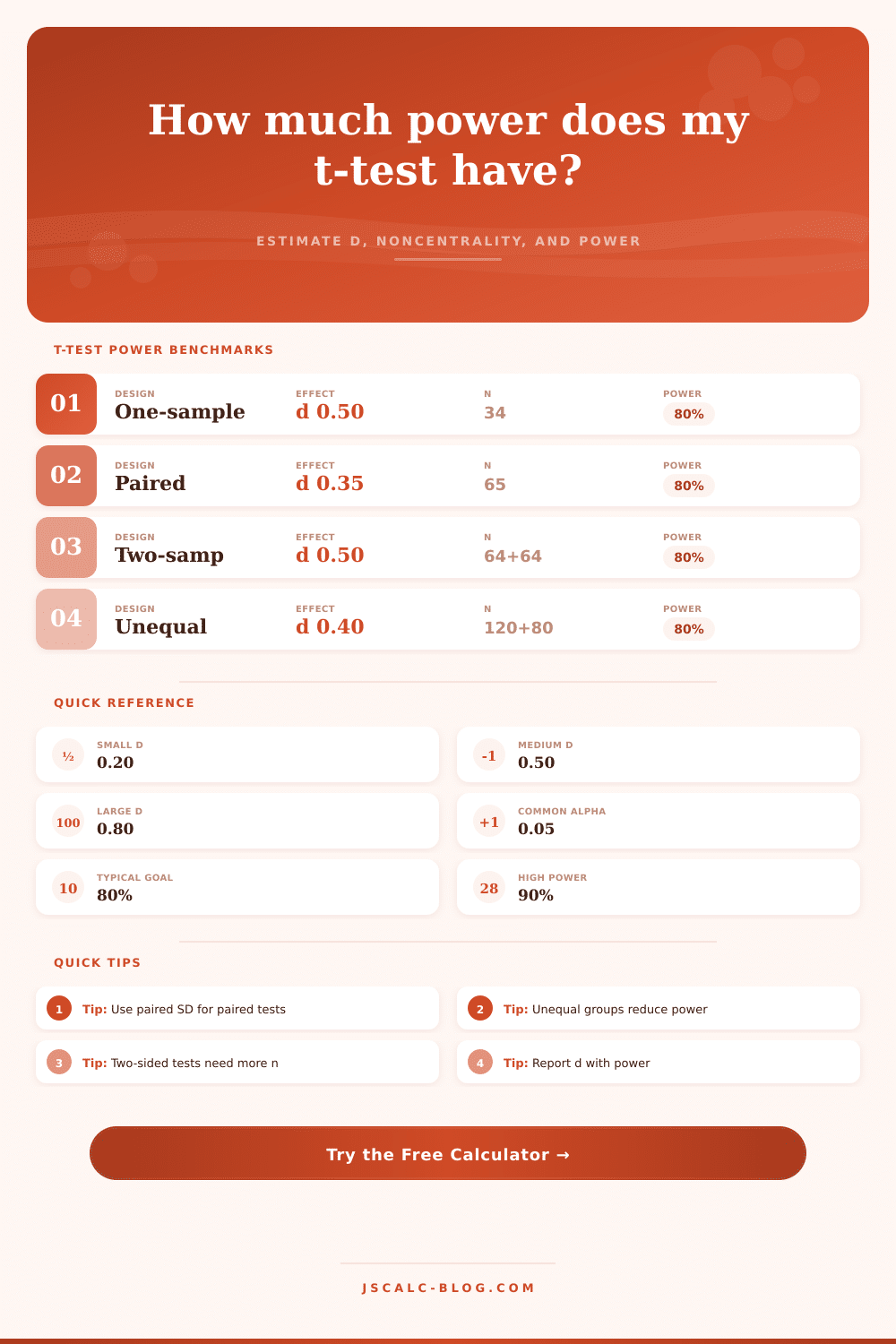
Medium paired change	Paired	0.50	0.05 two-sided	80%	About 34 pairs
Medium two-arm lift	Two-sample	0.50	0.05 two-sided	80%	About 64 per group
Large one-arm bias	One-sample	0.80	0.05 two-sided	90%	About 18 total
Small two-arm lift	Two-sample	0.20	0.05 two-sided	80%	About 394 per group
Directional paired test	Paired	0.35	0.05 one-sided	80%	About 51 pairs

🧮Critical Value Guide

df	0.05 One-Tailed	0.05 Two-Sided	0.01 Two-Sided	Notes
10	1.812	2.228	3.169	Small-sample tails are wide
20	1.725	2.086	2.845	Still meaningfully above z
30	1.697	2.042	2.750	Common pilot-study range
60	1.671	2.000	2.660	Near normal, but not identical
120	1.658	1.980	2.617	Large-sample behavior
Infinite	1.645	1.960	2.576	Normal z reference

📋Effect Size Interpretation Table

\|d\| Range	Common Label	Mean Shift Example	Power Impact	Planning Caution
0.10 to 0.19	Very small	1 to 1.9 SD tenths	Needs large n	Check measurement noise
0.20 to 0.34	Small	2 to 3.4 points if SD 10	Sensitive to tails	Avoid optimistic d
0.35 to 0.64	Moderate	3.5 to 6.4 points if SD 10	Typical feasible range	Use pilot SD if available
0.65 to 0.99	Large	6.5 to 9.9 points if SD 10	High power with modest n	Replicate assumptions
1.00+	Very large	10+ points if SD 10	Often high power	Watch selection bias

⚙Formula and Approximation Details

One-sample effectd = (mu1 - mu0) / sigma. Use this when one sample mean is tested against a reference value.

Paired effectd = mean difference / SD of paired differences. Do not use the raw baseline SD for a paired power calculation.

Two-sample effectd = (treatment mean - control mean) / pooled SD, using the common within-group standard deviation.

NoncentralityOne-sample and paired: delta = d x sqrt(n). Two-sample: delta = d x sqrt(n1 x n2 / (n1 + n2)).

Critical valueThe calculator estimates t critical from alpha and degrees of freedom using a Cornish-Fisher expansion around the normal quantile.

Power definitionPower is the probability that the test statistic falls in the rejection region under the alternative distribution.

Two-sided powerPower = F_nct(-tcrit; df, delta) + 1 - F_nct(tcrit; df, delta). One-tailed tests use the matching single tail.

Implemented approximationFor speed in WordPress, F_nct is approximated by a shifted normal distribution centered at delta with t tail variance df / (df - 2) when df is above 2.

💡Power Planning Tips

Effect-size tip: For paired designs, the SD must be the standard deviation of the within-person differences. A low before/after correlation makes that SD larger and lowers power.

Design tip: If a two-sample study must use unequal groups, keep the smaller group as large as possible. The noncentrality depends on n1 x n2 / (n1 + n2), so imbalance wastes information.

When study results aren’t quite statistically significant… Say your p-value was 0.06; power analysis can help you make sense off them. Maybe you had a clear goal for your study, recruited subjects, measured outcomes, and performed the analysis. You might then feel frustrated to see that your test isn’t significant even though it is very close to the line between significant and non-significant. Was there something wrong with your intervention? Or did you just miss picking up on the signal?

Power analysis give a sort of in-practice reality check for the way you designed your study. It tells you: were you able to pick up on the signal if there really was an effect? Fortunately, the math behind these non-central t-distributions is pretty complicated, but the calculator do all that math for you, letting you concentrate on decisions that make a real difference.

How to Use Power Analysis

Your initial entry is typically hardest. After all, how do you know how big an effect you are going to get? You have to make some guess about Cohen’s d. This is standardized difference between your groups, expressed in units of standard deviations. Standardization make it possible to compare differences in different type of measurements (e.g., changes in test scores with changes in blood pressure).

Because we’re humans who like to think positively, we frequently guess that the effect will be large, after all, then we don’t have to recruit many people! In reality, however, the effects tend to be much smaller than expected due to both biological variability and the fact that human are not always cooperative. Overestimating the effect result in underpowered experiments. Underestimating it results in wasted effort. Instead, try to use middle ground that you feel comfortabley defending. Review related published work or your own pilot data rather than hoping for outcome you want.

The second key choice involve the study design. Typically a two-sample independent test is not as powerful than a paired test (i.e., measuring the same individuals both pre- and post-treatment). Differences between people is eliminated in the paired design. It’s like comparing everyone with themselves; it controls for individual differences. The calculator consider the fact that you are using the standard deviation of the differences instead of just the standard deviation of baseline values. Many people make mistake of using the latter, thereby artificially increasing the necessary sample size. It’s a small detail but one that will save you from having to recruit too many participant.

The main way to control power is sample size. How many do I need? You typically aim for 80 percent or greater probability of detecting the effect you expect with reasonable confidence. In practice, bigger isn’t necessarily better. Time and money are required to recruit participants, and there are ethical guidelines suggesting we don’t run larger studies than are needed.

The non-centrality parameter, mentioned in the results section, indicates by how much the alternative distribution differ from the null. The more it differs, the farther away it will be located. That means it’s easier to see signal separate from noise. The problem is that you reach diminishing returns fast: Doubling your sample from 20 to 30 may double your power; doubling again from 50 to 60 might of give you just a few percentage points.

Inefficiencies arise from having unequal sized groups. When constraints force us into unequal groups, we lose some of our statistical efficiency compared to an equally sized design. The smaller group will drag down the performance of the bigger one because the effective power is determined by the harmonic mean of the two group size. Two moderately sized groups is preferable to one big group and another tiny.

In conclusion: Power calculation is humbling. It forces you to face the uncertainty of your numbers, the limits of your tools, and the cost of both before money is at stake. It makes the idea of “maybe” into something you can make real. And when you find yourself gazing at that 0.06 p-value, you’ll have some idea if it’s really a no (instead of “no, we couldn’t tell”) or yes.

It is not because the math guaranteed it, math never guarantees anything! It is because you set up the experiment correctly with the correct number of subjects and the right tools to detect what you think might be there.