Nyquist Sampling Rate Calculator
Find the minimum sampling frequency for any signal using the Nyquist theorem, where the Nyquist rate equals two times the highest frequency component. Compute the Nyquist folding frequency at half the sampling rate, the oversampling ratio, and a recommended sampling rate with a guard band for anti-alias filter roll-off, or check whether a chosen fs is adequate.
🔊Choose a Mode
🎯Real Signal Presets
📝Signal & Sampling Inputs
Highest frequency component present in the signal.
Unit applied to the maximum frequency above.
The sample rate you plan to use, for checking or fs/2.
Unit applied to the sampling rate above.
Extra headroom above 2 x f_max for filter roll-off.
A tone of interest, in the same unit as f_max.
Resolution per sample, used for the data rate.
1 for mono, 2 for stereo, more for arrays.
Controls rounding on every result card.
🔢Formula Snapshot
📋Max Frequency to Nyquist Rate
| Max Frequency f_max | Nyquist Rate = 2 f_max | Common Practical fs | Reads As |
|---|---|---|---|
| 50 Hz | 100 Hz | 128 Hz | Slow biosignal |
| 500 Hz | 1 kHz | 1.25 kHz | Vibration sensor |
| 3.4 kHz | 6.8 kHz | 8 kHz | Telephone voice |
| 15 kHz | 30 kHz | 32 kHz | FM baseband |
| 20 kHz | 40 kHz | 44.1 kHz | Hearing limit |
| 22.05 kHz | 44.1 kHz | 48 kHz | Studio audio |
| 100 kHz | 200 kHz | 250 kHz | Sonar ping |
| 1 MHz | 2 MHz | 2.5 MHz | RF IF stage |
| 5 MHz | 10 MHz | 12.5 MHz | Ultrasound |
📊Oversampling Ratio Guide
| Ratio fs / 2 f_max | Status | Filter Effort | Typical Use |
|---|---|---|---|
| Below 1.0 | Aliasing | Impossible | Under-sampled, avoid |
| 1.0 exactly | Critical | Brick wall | Theoretical limit only |
| 1.1 | Tight | Very steep | Bandwidth limited links |
| 2.2 to 2.5 | Comfortable | Gentle roll-off | Most audio and DAQ |
| 4 to 8 | Relaxed | Simple filter | Delta-sigma converters |
| 16 to 64 | Heavy | Digital decimation | High resolution ADCs |
| 256 and up | Extreme | Trivial analog | Audiophile DACs |
🎵Standard Sampling Rate Comparison Grid
| Standard fs | Nyquist fs/2 | Usable f_max | Bit Depth | Channels | Data Rate |
|---|---|---|---|---|---|
| 8 kHz | 4 kHz | 3.4 kHz | 8 bit | 1 | 64 kbit/s |
| 16 kHz | 8 kHz | 7 kHz | 16 bit | 1 | 256 kbit/s |
| 32 kHz | 16 kHz | 15 kHz | 16 bit | 2 | 1.02 Mbit/s |
| 44.1 kHz | 22.05 kHz | 20 kHz | 16 bit | 2 | 1.41 Mbit/s |
| 48 kHz | 24 kHz | 22 kHz | 24 bit | 2 | 2.30 Mbit/s |
| 96 kHz | 48 kHz | 45 kHz | 24 bit | 2 | 4.61 Mbit/s |
| 192 kHz | 96 kHz | 90 kHz | 24 bit | 2 | 9.22 Mbit/s |
| 2.5 MHz | 1.25 MHz | 1 MHz | 12 bit | 1 | 30 Mbit/s |
| 12.5 MHz | 6.25 MHz | 5 MHz | 12 bit | 1 | 150 Mbit/s |
📏Frequency Unit Conversions
| Unit | Equals | In Hertz | Note |
|---|---|---|---|
| 1 Hz | 1 cycle/s | 1 Hz | Base unit |
| 1 kHz | 1000 Hz | 1000 Hz | Kilohertz |
| 1 MHz | 1000 kHz | 1000000 Hz | Megahertz |
| 1 GHz | 1000 MHz | 1000000000 Hz | Gigahertz |
| 1 rad/s | 0.159 Hz | 0.159155 Hz | Divide by 2 pi |
| 1 rpm | 0.0167 Hz | 0.016667 Hz | Cycles per minute |
⚙Formula Breakdown
💡Practical Sampling Tips
But then you connect it to an analog-to-digital converter. Your pretty analog signal gets converted to an ugly digital one. There’s all this nuance and detail, and now there are these jagged stair steps of a waveform. And then whole incorrect frequencies materialize out of thin air! That’s when the Nyquist theorem goes from abstract math to something with real-world consequences: the difference between useless data and a useable recording.
The math gets done for you by the calculator above. You can concentrate on whether or not your hardware decisions makes any sense. It knows your highest frequency. It converts it to a tangible lowest sampling rate. Knowing what it is is every bit as important than understanding why it is.
How to Pick the Right Sampling Rate
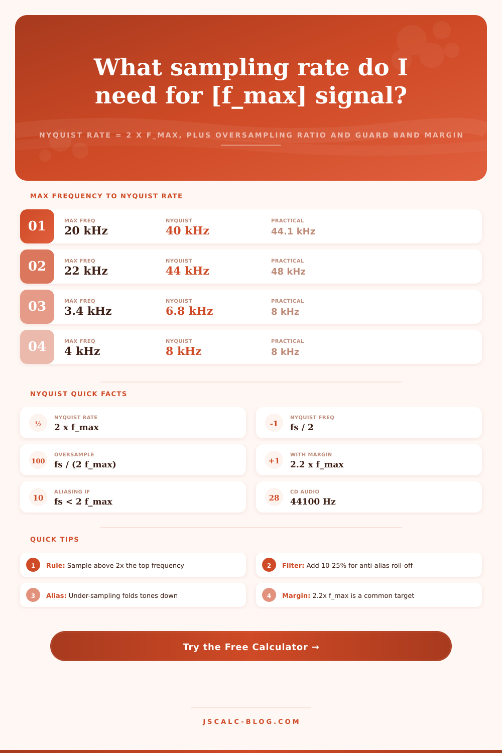
It’s simple enough to stick on a sticky note. You must sample at twice or more than the highest frequency in your signal. If your audio tops out at 20 kilohertz, you want a sampling rate above 40 kilohertz. That’s called the Nyquist rate. Go below it and aliasing happens.
Higher frequencies will fold back into the audible range. They sound like a phantom tone. It was a tone that was never there to begin with. And once they’re caught, they can’t be filtered out later. Now they’re just real signal data. Anything that tries to cross the mirror of its folding frequency, which is half your sampling rate, bounces back down the other side. Everything that wants to cross over folds back down the other side.
So for all digital systems, knowing your bandwidth limit is the first step in designing anything. Theoretically speaking, it’s rare that this are practical. In the real world, there isn’t some magical wall when signals cross frequencies. The signal fades gradually over time. And if you sample a signal at precisely 20 kilohertz, but your sampling rate is only 40 kilohertz, then your filter would of gone from 100% down to 0% immediately. That’s just not possible with normal components.
That’s why the tool recommends a guard band and offers an oversampling ratio. One means you’re on the edge, exactly. Two or more means you’ve got some breathing room for your analog component. The recommended rate is a percentage above theoretical floor as a safety margin. Ten percent is a good place to start. This allows the filter to work within a transition zone. It gives the filter time to work without getting too close to the signal near the cutoff.
There are always tradeoffs with a standard rate. When recording compact disc audio, we use 44100 Hertz. Our content goes up to 20 kilohertz. That means there’s only about two kilohertz of headroom left before the anti-alias filter fades off. To achieve a gentler slope, studio systems jumps up to 48 kilohertz or better. Telephone voice is just 3.4 kilohertz or so and sampled at 8 kilohertz. It fits easily in available transmission slots without wasting bandwidth.
Every application has its own balance of fidelity, cost, and storage. Ultra-high fidelity audio may go as high as 192 kilohertz in order to push the quantization noise way out of band. Medical sensors that sample heart rates don’t need ultra high frequency response as much as they do stability. You can toggle between these modes on the calculator. It will show you where your particular signal falls within commonly used standards.
You might be tempted to double your sample rate and go on about your business, but when you check the next column, the data rate column, higher numbers start to raise some red flags. If you double the number of samples, you double the amount of work for your processor and double the amount of space required to store results. It demands more from your memory buffers and more from your converters.
You probably won’t need those high rates for a sensor that takes slow changing temperature measurements. You will if you’re creating ultrasound images, or sending out radar pulses, where each microsecond matters. The channel count and bit depth quickly compound this impact. At 16-bits per sample with two channels at 44,100 samples per second, that’s more than a million bits per second. That’s what you pay for clarity.
You’re not looking for max; you are looking for good enough. Let the tool tell you where that is. Find that sweet spot where your signal sits comfortabley just below the fold point. Give your filter some space to operate. Compare your selected rate with the Nyquist limit. Inspect carefully for any aliases hiding in the background. A little breathing room is a long ways from having dirty data.
Once you know how fast your sampling clock ticks relative to the highest end of your signal, those jags goes away. Those stairs step back down to reveal the original curve once more. You’ve caught the signal’s real form, free from the noise of poor design.